Appendix 2.1: Alternative ways for the modeling of LDSs

The operationalization of the conceptual and interpretative framework for SHD at the local level requires moving beyond standard analytical method­ologies. For instance, Schmiedeberg (2010) underlines how econometric methods (such as difference-in-difference), and particularly spatial econo­metrics, can quantitatively test the effects of local development policy.

However, data requirements and methodological standards are high, and often fail to take adequate account of soft factors (Maggino and Nuvolati, 2011). Moreover, in cases of territorial differences and place-based processes, econometric estimates regarding firms' performance or people's well-being (among other things) may be biased if multilevel analysis is not conducted.

Without any intention of exhaustiveness, the aim of this appendix is to briefly introduce six methodologies for alternative ways of modeling that can help make the STEHD framework advanced in this book operational. These methodologies share a common feature: flexibility. Furthermore, they can introduce qualitative variables as explicative determinants, as well as, for the first two methods, descriptive factors as an integrated part of modeling. Nonetheless, applying these methodologies may require specific statistical assumptions and is demanding in terms of time and resource, especially if data needs to be collected.¹⁶

Agent-Based Modeling and computational economics

Agent-Based Modeling (ABM) and Simulation (ABMS) is a relatively new approach to modeling economies as complex adaptive systems in sys­temic and non-linear analysis. These systems are composed of interacting, autonomous “agents” who interact with and influence each other, learn from their experiences and adapt their behaviours so that they are bet­ter suited to their environment (Nelson and Winter, 1982; Lombardi and Squazzoni, 2005; Macal and North, 2010).

The application of ABM to LDSs provides a useful analytical tool for investigating territorial evolution and for understanding mechanisms and processes relating to local development and institutions that enable capa­bility expansion (see for instance Brenner, 2001; Lombardi, 2003; Lombardi and Squazzoni, 2005).

According to Andersen (1994), the main epistemic assumptions of ABM are as follows:

1) Agents have incomplete information and tend to satisfy local rather than global optimality criteria.

2) Systemic institutional causes limit the decision-making processes.

3) Imitation, learning and creation of novelty are fundamental processes.

4) Path dependence, together with potential discontinuity traits, shape dynamic processes.

5) Interaction among agents and disequilibrium are strongly interconnected.

6) The dynamic results that ensue are non-deterministic, open and irreversible.

Data Envelopment Analysis

Data Envelopment Analysis (DEA) is a flexible non-parametric mathemati­cal model for the management and assessment of the technical efficiency of social organizations in relation to their size and resources. Key advantages of this technique include a multi-input/multi-output approach, indifference to the measuring unit of the considered variables and avoiding specific ex-ante assumptions about the shadow prices of inputs and outputs (Charnes et al., 1978). Bellucci et al. (2012) utilize DEA for the calculation of a "socio­cultural efficiency frontier” going beyond the standard economic frontier, while Binder and Broekel (2011) have applied it in relation to individual conversion factors and functionings within the CA.

The first model introduced by Charnes et al.

As regards to the output-oriented version of the BCC model, it is possible to write the maximization problem in the following way:

Under the constraints:

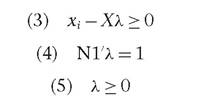
with 1 < 0 < to and 0 — 1a scalar representing the proportional increment of output that the z-th decision-making unit could achieve maintaining con­stant inputs; k representing a N x 1 vector of constants; x representing the input data matrix; and Y the output data matrix.

Consequently, the technical efficiency score is defined by 1/0 and can vary between 0 and 1.

Social Network Analysis

Social Network Analysis (SNA), rooted in graph theory, is based on the assumption that relationships among interacting actors are important to explain development processes and institutions (Bellandi and Caloffi, 2010). Watts and Strogatz (1998) formulate a mathematical model describing sys­tems with "small world properties”. These systems have two core properties: (i) high local density, as actors have dense connections with their neigh­bours; and (ii) few connections with other distant actors (Giuliani and Pietrobelli, 2011, p. 14).

Relational data, represented in two-way matrices, is critical for network data (see Giuliani and Pietrobelli, 2011 for several empirical examples). A network is considered as a finite set (or sets) of actors and the relations the define them. An actor is a discrete individual, corporation or other organizational unit, such as people, associations, firms, research institutes, universities and government agencies. Social ties link the actors together and each actor is identified as a node in the network.

As Wasserman and Faust (1994) illustrate, SNA differs from standard social or behavioural science methods, viewing characteristics of the social units as arising out of the structural or relational processes and focusing on proper­ties of the relational systems themselves, which are crucial in analysing LDS within an SHD perspective.

Structural Equation Modeling

Economists have begun to apply Structural Equation Modeling (SEM) in order to measure latent concepts, such as institutional changes and tech­nological capabilities. According to Hox and Bechger (1998), SEM can be understood as a combination of factor analysis and regression or path analy­sis. The basic idea is that, after relationships of interest variables are defined, latent variables¹⁸ can be estimated by the relation to observed variables (multiple indicators).

The SEM theoretical construct on the latent factor can follow the frame­work flow, and it implies a structure of co-variances between the observed variables. It can be visualized by a graphical path diagram, showing indirect and direct pathways.

SEM can be applied to the CA in order to measure a specific individual capability basing the measure on observable functionings and personal char­acteristics (Kuklys, 2005; Di Tommaso, 2007; Krishnakumar and Ballon, 2008). In addition, SEM can be applied in order to examine complex rela­tionships between observed and latent variables such as opportunities to function or functionings at territorial level in terms of SHD.

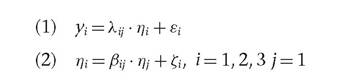
where y_i are the observed variables, while the latent variables (agglomera­tion economies, quality of life /labour, urban infrastructure) are symbolized with nZ the m variable is the latent factor of "firm competitiveness”; k_ii are the factor loadings indicating the effect of the latent variables on the observed indicators, while e_i, are the measurement errors that are assumed to be uncorrelated between measurement equations with nd and Z repre­senting measurement errors in the structural equations, respectively, and ß, denoting factor loadings indicating the effect of the three latent variables upon "firm competitiveness”.

The scale of latent factor "firm competitiveness” is fixed by assuming that it has a unit variance. It is also hypothesized that: E(£_t) = 0, Cov(Z_i, nt) = 0, Cov(et, Zi) = 0.

The results show that firms' competitiveness in the territory - the latent factor - is strongly and positively related to all three latent variables.

Scenario Analysis

A scenario describes (textually or graphically) a set of events that might rea­sonably take place. Scenarios can be considered as hypothetical images of the future, which describe the functioning of a system under different con­ditions with a certain degree of uncertainty. Kahn and Wiener (1967, p. 3) originally defined scenarios as ‘hypothetical sequences of events constructed for the purpose of focusing attention on causal processes and decision­points'.

(Bunn and Salo, 1993). One of the main advantages of scenario analysis with respect to standard statistical forecasting techniques is that it can be used to consider the impact of future exogenous shocks and major structural changes in the system under analysis. Scenario based on expert assessment can however benefit from a structuring processing of the elicited informa­tion, e.g. using network analysis and methods to verify the consistency and accuracy of expert assessments (Gambelli et al., 2010).

Bayesian Networks

A Bayesian network is a compact probabilistic model for the handling of uncertainty in expert systems (Jensen, 1996). It can be interpreted as a graph­ical model of the interactions among a set of variables, and a set of directed edges between variables, where each variable has a finite set of mutually exclusive states. The resulting network should have a Directed Acyclic Graph (DAG) format, i.e. a graph with no directed cycles among nodes. Each node A is associated to a conditional probability table P(A|B₁,..., B_n), where B₁,...,B_n are parents nodes of A, i.e. nodes upon which A is dependent.

The advantage of this approach with respect to standard econometric tools (e.g. discrete choice models for risk evaluation) is the possibility to consider the cumulative effects on risk due to a combination of risk factors, and that qualitative evaluation of utility can be considered. Bayesian networks can be designed from hard statistical data using specific “learning” algorithms, or based on expert knowledge. Among many other fields and examples, here we just mention the potential of Bayesian networks as decision support, when integrated with a utility function (Cowell et al., 2007), and for risk evaluation (Gambelli et al., 2014).