Modeling Credit Markets

One of the core assumptions of the neoclassical model is that there is a single market interest rate and every firm invests to the point where their marginal product is equal to this rate.

Perhaps the most direct evidence comes from attempts to estim­ate the marginal product of capital. McKenzie and Woodruff (2003) estimate parametric and nonparametric relationships between firm earnings and firm capital in Mexico. Their estimates suggest that the return on capital for firms with less than US $200 invested is of the order of 15% per month. For firms with investment between US $200 and US $500 the return is between 7% and 10% per month, and it goes down to 5% for firms with investment between US $500 and US $1,000. All of these are well above the informal interest rates available in this area in pawn shops or through micro-credit pro­grams (on the order of 3% per month). In other words, none of the estimated marginal products are equal to each other or to the rate that best approximates the market interest rate.

There are however obvious methodological issues with studies of this kind. First, the investment levels are likely to be correlated with omitted variables. For example, in a world where people can borrow as much as they want, investment will be positively correl­ated with the expected returns to investment, generating a positive “ability bias" (Olley and Pakes 1996). McKenzie and Woodruff attempt to control for managerial ability by including the firm owner's wage in previous employment, but this may only go a part of the way if individuals choose to enter self-employment precisely because their expected productivity in self-employment is much larger than their productivity in an employed job.^[II]

Others take a more indirect approach to this problem.

However, this approach has its own problems. The main issue is whether shocks to cash flow are proxying for shocks to the firm's productivity. Fazzari et al. (1988) show that their results do not change when they include controls for the firm's market value, which ought to pick up any changes in the firm's productiv­ity. A concern remains however that the market may not know everything that one needs to know about the firm's productivity.

Lamont (1997) addresses this issue by using cash flow shocks that come from an identifiable source, namely shocks to the price of crude oil. He then looks at what happens to the non-oil invest­ments of companies that own an oil company and finds a strong cash flow effect. However, given how big the oil companies are, it is possible that this response has nothing to do with credit con­straints, but rather reflects managerial behavior in the presence of “free cash flow."

Banerjee and Duflo (2004) take a yet different approach. They observe that an implication of being unconstrained in the credit market in the sense of being able to borrow as much as you want at the market rate, is that the inflow of subsidized credit into a firm should cause the firm to pay down its nonsubsidized debt, before undertaking additional investment. A constrained firm, by con­trast, will want to put what it gets into fresh investments, because its marginal product of capital is higher than the market rate.

To operationalize this strategy they take advantage of a change in the definition of the so-called “priority sector" in India to gen­erate a “natural experiment."All banks in India are required to lend at least 40% of their net credit to the “priority sector,"which from the traditional maize and cassava intercrops to pineapple is estimated to be in excess of 1,200%! Few people grow pineapple, however, and this figure may hide some heterogeneity between those who have switched to pineapple and those who have not.

includes small-scale industry, at an interest rate that is required to be no more than 4% above their prime lending rate. In January 1998, the limit on total investment in plants and machinery for a firm to be eligible for inclusion in the small-scale industry cat­egory was raised from Rs 6.5 million to Rs 30 million. Banerjee and Duflo first show that, after the reforms, newly eligible firms (those with investment between Rs 6.5 million and 30 million) received on average larger increments in their working capital limit than smaller firms, both in absolute terms and relative to preex­isting trends. They then show that the sales and profits increased faster for these firms during the same period. In particular, sales increased almost as fast as credit, suggesting that almost no one is using the extra money to pay down their debt. Most firms appear to be credit constrained.

Banerjee and Duflo then use the variation in the eligibility rule over time to construct instrumental variable estimates of the impact of working capital on sales and profits. The elasticity of profit with respect to working capital is almost 2. Using this and making allowances for the subsidy element in the cost of capital, they estimate that the returns to capital in these firms must be at least 90%. The market interest faced by these firms is certainly no more than 3% per month (43% per year), which is consistent with the rest of the evidence on the firm's being credit constrained.

There seems to be clear evidence that the typical firm, at least in the developing world, has a marginal product which is sub­stantially above the market interest rate. This suggests that the firm cannot borrow as much as it wants at the going market rate. In other words, the supply curve of capital to the firm must be upward sloping, or even vertical (a hard limit on how much the firm can borrow).

To end this section we sketch a simple model taken from Aghion et al. (1999a) that explains why lenders impose limits on how much firms can borrow.

Consider a borrower who needs to invest W + L = I in a high- yield technology, where W denotes his or her initial wealth and L is his or her requested loan. The interest rate is r. Both the bor­rower and the lender are risk neutral. The source of capital market imperfection is the possibility that the borrower may choose not to repay. Namely, once the return F(W + L) is realized, the bor­rower can either repay immediately and get a net income equal to

F (W + L) — rL, or he or she can stall. Stalling revenues away from the lender has a cost to the borrower (who has to keep ahead of the lender); let this cost be a fixed proportion τ of the total investment. Finally, whenever the borrower defaults on his or her repayment obligation, the lender may still invest effort into debt collection. Specifically, assume that a lender has a probability p of collecting his or her due repayment rL. Assume F (W + L) — τ(W + L) > rL (so that if the borrower stalls but is caught, he or she still has enough resources to repay the lender). Also, take r as exogenously given.

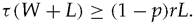
For any given p, the borrower faces a choice between honoring the debt contract and getting F (W+L)—rL, and stalling and getting an expected income of F(W + L) — τ(W + L) — prL (because he still gets caught with probablity p). He will choose the more honorable option if and only if

which implies that

From this it follows that the amount the lender will be prepared to lend (assuming that he wants the borrower to repay) is capped

The amount lent is proportional to the borrower's wealth, increas­ing in the cost of stalling, decreasing in the interest rate, and increasing in the probability of making the borrower repay.

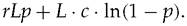
However, it is not clear whether it is reasonable to assume that p is exogenously given: Those lenders who have a greater stake in getting the borrower to repay, will presumably try harder, and therefore p will depend on the amount the lender hopes to get back. To capture this idea, assume that once the borrower starts stalling the lender faces a choice: He can guarantee himself a probability p of collecting his or her due payment rL incurring a nonmonetary effort cost L ∙ C(p), where C(p) = —c ∙ ln(1 — p).

Faced by a borrower who is stalling, the lender will choose p to maximize:

The optimal choice of p is the one for which

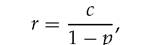
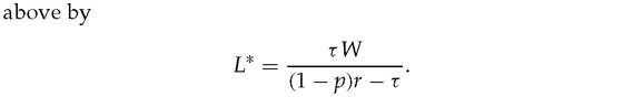
or r(1 — p) = c. It follows that the credit limit, L*, will be given by

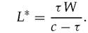
Note that this is proportional to the borrower's wealth, and increasing in τ, the cost of cheating the lender, and decreasing in c, which determines the lender's cost of collection. This model suggests that the ratio of τ to c, representing the ratio of the cost of cheating to the cost of apprehending cheaters, is a natural measure of the level of financial development. Lending, not surprisingly, is increasing in τ∕c.

In the rest of the book, when we simply assume that firms are credit constrained, and the constraint takes the form L ≤ μW, where μ is a positive constant that is increasing in the level of financial development, we will have in mind the model in this section.