Similarities of Trading Strategies Between SF Spread and Random Strategy
4.4.1 Arbitrage: Equalization Between Markets
Profit-seeking activities will make different situations more similar. This is called “arbitrage”:
• If the spot price is higher than the futures price, then buy futures and simultaneously sell the same amount in the spot market.
• If the position of both markets is kept fixed until the settlement date, very little loss will be incurred, because settlement is conducted using the same price (the spot price) to the same positions. If the spot price falls rapidly (spot price > future price, or the SF spread is too large), profits will be made.
4.4.1.1 The Essence of Arbitrage
Arbitrage is one of the most important mechanisms to intermediate different kinds of market. Here, we focus on arbitrage between the spot and futures markets, where it may be defined as the management of the short and long positions, which is effectively risk management on trading.
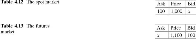
Historically, when he commented on Hayek’s idea of the natural rate of interest, Sraffa (1932a,b) using arbitrage, cleverly explored how there was no such unique rate in the market. Sraffa’s idea is easily illustrated using the order book. Sraffa considered the trade in bales of raw cotton, but only the so-called “day trader’s method”, the implementation of simultaneous alternative moves, i.e., cross trades of ask in the spot market and bid in the futures market, or bid in the spot market and ask in the futures market.6 The next numerical example uses the cross trades of ask in the spot market and bid in the futures market:
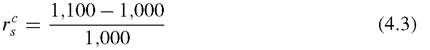
In this case, settlement in both markets could be feasible if x was implemented. In this case, the concerned trader can earn U10,000(= 1,100 — 1,000 x 100 bales). The self-interest rate is therefore calculated as (Tables 4.12 and 4.13):
6Given a single market, this may be simultaneous ask and bid.
The rate of interest is a personal rate, which is connected with an intertemporal rate common to the traders whose operation can be established directly in the market. Sraffa called this “the commodity (cotton) rate of interest”. This definition can be generalized to many other commodities with their own market both for spot trades and futures. It is also clear that there are as many commodity rates of interest as there are commodities.
Sraffa criticized Hayek’s naive opinion that a single natural rate of interest could exist. Hayek was not successful in formulating a credit system. He did not understand that there were multiple commodity rates of interest, or how such multiple rates could be equalized. The equalization never holds automatically. Implementing it requires a particular mechanism of credit allocation to appropriate investment funds for traders, as well as a particular institutional deployment. We have already learned that the market mechanism always underlies institutional formation. Without understanding the effects of the current institutional framework, no innate force can emerge, as Hayek imagined for the natural rate of interest.
We can compare Sraffa’s objective definition with Fisher’s subjective one[55]:
Irving Fisher carried out work in the 1930s to define the ‘own’ rate of interest. He intended to derive it directly by the subjective motivation of consumption. The ‘own’ rate of interest of an apple for a consumer is interpreted as the exchange rate of today’s apple at with tomorrow’s apple atC1. By this definition, on the surface, the subjective rate of temporal exchange seems to hold, as does the idea that tomorrow’s apple should be appreciated more than today’s because it has been earned by giving up a part of today’s. The difference between αt and αtC1 may then be expected to be the sacrifice equivalence for the consumer of today, to reserve it for tomorrow.
The subject’s inner preference therefore decides the ‘own’ rate of interest. This also seems to support the next relation:
However, the converse relation never gives a natural meaning of patience. It rather refers to wasting. We therefore need to force the former relation to be held by introducing the evaluation of the discounted price system. The discounted price, by definition, is always decreasing over time. If we employ the current prices Pt, then the number of apples purchased by ¥1 at date t, i.e., αt, and the number of apples purchased by ¥1 at date t C 1, i.e., αtC1, are defined as:
(continued)
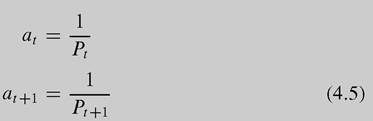
If the apples are purchased by borrowing money at the money rate of interest rm, it then holds that:

It is then trivial that the ‘own’ rate of apples rα may be negative if the part Pt — Pt+1 of the numerator is negative.
If the market works freely, the subjective meaning of the intertemporal rate could be lost. This method can neither stand by itself nor adapt to the market. The meaning of the own rate of interest does not cause any difficulty, even when negative, if Sraffa’s method is employed. This is a natural outcome of the market mechanism. As the market fluctuates, the rate of exchange also changes in terms of price. The price may be down tomorrow, and then the own rate must be negative.
In the past, economists often insisted that there was an easy connectivity between intertemporal choices between the consumption and transformation sets of production, to give a kind of intertemporal equilibrium. However, this connection will never be generated by the arbitrage mechanism working through the markets, and this thinking results in a false sense of reality.
As stated at the beginning of this section, the function of arbitrage in the spot and futures markets will imply the need for position management for the traders. Arbitrage of this kind can also cause discrepancies between multiple commodity rates of interest, whether positive or negative. We now consider the working of arbitrage in a special example.
4.4.1.2 SF Spread Strategy and Arbitrage
SF spread represents the distance between the spot price and the futures price.We now consider arbitrage between the spot and futures markets. The agent orders when a spread between spot and future price is wider than the threshold. If the future price is higher, the agent gives a buying order, and if it is lower, a selling order (Fig. 4.9).
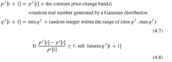
The order price is given by a Gaussian distribution whose mean is set as the latest future price pf [t] and whose standard deviation is set as the price change band triangle. Order volume is a uniform random number between min qf and max qf.
Fig. 4.9 SF spread
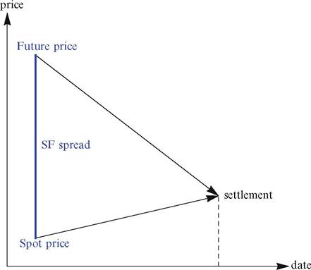
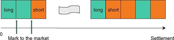
Fig. 4.10 Canceling out the positions. On average during all trading days, the blocks of long and short positions will tend to be canceled out
4.4.1.3 Random Strategy
The agent buys or sells randomly. The limited price on order is set randomly around the latest price, and quantity is set randomly within a prescribed range. Either position of the agent is also limited to the upper limit.
SRandom: employ the latest spot price
FRandom: employ the latest futures price
If the random strategy is not successful in any particular session, the order is held over to the next session, and kept as a position in either direction (short or long). The sessions therefore accumulate the position until the end of the day, when the mark to the market is executed. Each day will have either a short or long position.
On average during the whole trading period, the positions will be canceled out (Fig. 4.10).| Ask | Price Bid | |
| 82 | 1798 | |
| 73 | 1793 | |
| 38 | 1779 | |
| 44 | 1778 | |
| 91 | 1776 | 67 |
| Jm770 | 6 | |
| 93 | 1763 | 6 |
| 57 | J1759 | 23 |
| 1758 | 71 | |
| 1741 | 71 | |
| 1733 | ||
| 1729 | ||
| 1719 | ||
| 1684 | 31 | |
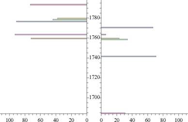
Fig. 4.8 Left, partial revision of daily price limits and special renewal price intervals; right, Itayose matching
4.4.1.4 Similarities Between SF Spread and Random strategies8
The agent decides whether to fewy[0], seZZ[1], or donothing[2] according to 0,1,2 randomly generated. No order is given if qf [t C 1] generates a result exceeding the given prescribed position. The size of the short and long position is limited.
This inequality is then equivalent to:

Here v is an arbitrary threshold.
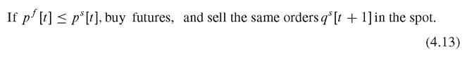
We can define the ‘buy’ condition as:
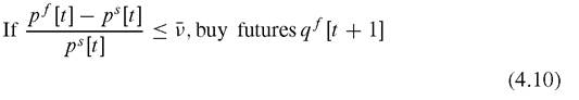
This inequality is then equivalent to:

Here v is also an arbitrary threshold.
In this market system of spot and futures, arbitrage between the spot and futures markets may be defined as: 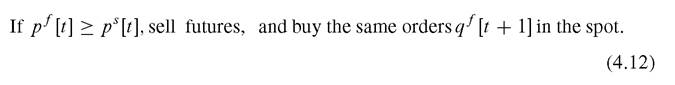
8This part depends on Kita (2012). Prof. Hajime Kita, Kyoto University, has recognized this fact and arranged well the U-Mart Project of a simple shaped market at the beginning of this project. The description of this subsection depends on his discussion.
These numerators exactly correspond to the conditions for arbitrage. It is therefore clear that the SF spread strategy is essentially equivalent to arbitrage between the spot and futures market.
4.4.2 The Performance of the Random Agents
in U-Mart ver. 4's Simulation
U-Mart deals with the futures trade, at present, by taking into account spot market motion. Usually, for the convenience of traders, the spot market price data are extrapolated into the GUI screen. We arrange technical agents of both types, whether the reference price series used to forecast the future market motion is that of spot (S type) or future prices (U type). Here, we consider two kinds of experimental design to examine the effects of random agents. Random agents in U-Mart are classified into two types: SRandomStrategy, which randomly gives orders around the spot price series, and URandomStrategy, which gives orders around the futures price series. We use the default setting for experiments, with two sessions per day over 5 days, depending on the TSE session time allocation in Fig. 4.11. We also use the same spot price series chosen in the default data set.9
Case 1 experiment We use a set of technical agents: URandomStrategy (5 units), SRandomStrategy (5 units), UTrendStrategy (1 unit), STrendStrategy (1 units), UAntiTrendStrategy (1 units), SAntiTrendStrategy (5 units), URsiS- trategy (1 units), SRsiStrategy (1 units), and UMovingAverageStrategy (1 units), UMovingAverageStrategy (1 units).
Case 2 experiment Here, we limit the agent types to a random strategy: URan- domStrategy (5 units) and SRandomStrategy (5 units).

Fig. 4.11 TSE's session time allocation
[1]Our spot time series is adapted from ‘2009-5-25_2010-1-6.csv’ in src/nativeConfig in the U-Mart ver. 4 system.
4.4.2.1 Case 1: Including Technical Agents Apart from Random Ones
In our custom, the trade volume in the futures market is in the plane measured by the vertical axes on the right-hand side. The peak values of transaction repeated alternatively from each cycle of 120 to each 150 units of time. These figures just are established by the TSE session time allocation, shown in Fig. 4.11.
Our results reveal a good performance of SRandom in comparison with URan- dom strategies. This may reflect the situation when the futures price series is generated around the spot price one. If this were the case, the probability of stipulation would be increased. A higher rate of stipulation does not necessarily guarantee profit, but may increase the changes of a profit in the Zaraba or double auction. When the futures price moves more than the spot price series, the agent working on the basis of the futures price may not only have less chance to make profit, but also suffer a higher probability of being matched by others at a very adverse rate. In the U-Mart experiments, then, the SRandom strategy will usually achieve a much better performance than the URandom one.
We already noted that both cases had the same spot market implementation for both simulations. In both cases, the SRandom group performed better than the URandom one. This shows that the average profit of the SRandom strategy group is much higher than that of the URandom strategy group. All the URandom agents, but only one SRandom agent, recorded negative profits (Fig. 4.12).
4.4.2.2 Case 2: A Comparison of Performance Between SRandom and URandom
In Case 2, if we examine the position management for each agent, SRandom agent 1, who suffered from a consequential loss, behaved as if there was no intelligent position management at all. The cross-section between total buy and sell, which is equivalent to a loss-cut, appear about eight times. The loss to SRandom agent 1 is estimated to be less. Similar reasoning can be applied to URandom agent 4, who suffered least, and to SRandom agent 3 and URandom agent 5 in Case 1 (Figs. 4.13 and 4.14).
We suggest that SRandom agents like 2 and 4, who are committed to position management, secured big profits because at the settlement date in this experiment, the spot price exceeded the futures price. The situation therefore favors those agents whose total buy is greater than their total sell. They can then resell the excess buy at a higher spot price to confirm the excess profit.
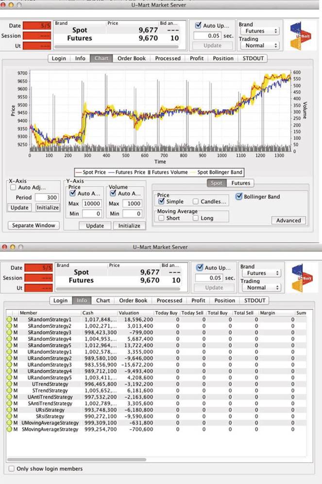
Fig. 4.12 Case 1 Experiment. Note: The highlighted band around the spot price line represents ‘Bollinger band’, which is a ‘technical analysis tool’ invented by John Bollinger in the 1980s
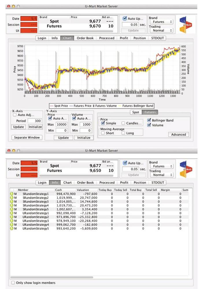
Fig. 4.13 Case 2 Experiment
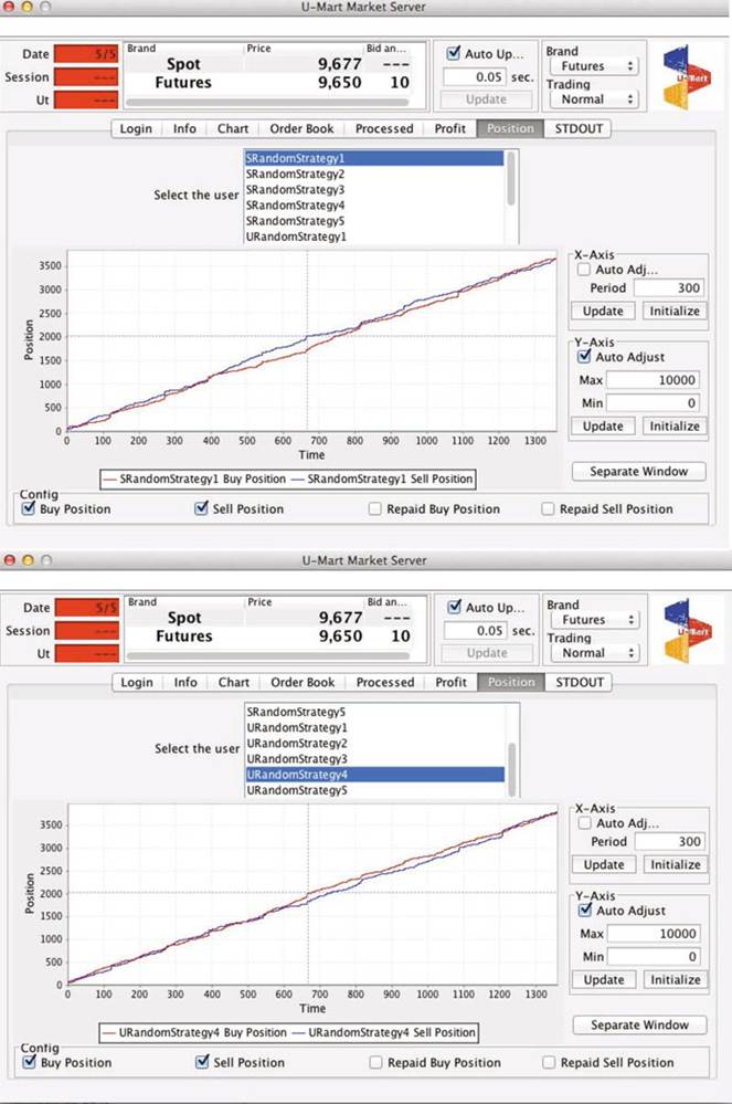
Fig. 4.14 Case 1 Position managements of random strategies