DATA ANALYSIS
Partial least squares (PLS) approach was developed in the 1960Æs by Herman-Wold as an econometric technique. Basically, PLS is similar to regression analysis, but it is capable of latent variable modelŁing and offers causal modeling techniques that have made it possible for researchers to examine the theory and its measures simultaneously.
AdditionŁally, PLS is appropriately used under conditions of non-normality and small to medium sample sizes (Chin & Newsted, 1999). Hence, we use PLS to perform the data analysis. The computer program used for this analysis was the Smart PLS 2.0. The bootstrap re-sampling method with re-samples of 900 determined the significance of the paths within the structural model.Reliability and Validity
First, construct reliability and validity were estabŁlished using confirmatory factor analysis (CFA) (Figure 2). Convergent validity was evaluated for the research model according to criteria recomŁmended by Fornell and Larcker (1981). These are: (1) Construct reliability in terms of composite reliŁability (CR), defined as the internal consistency of the indicators measuring a given factor exceeding 0.80, and (2) the average variance extracted (AVE) from each construct should exceed 0.50. AVE asŁsesses the amount of variance that is captured by the underlying factor in relation to the amount of variance due to the measurement error. Based on the calculations (Table 3), the results show that the composite reliability of each factor is above recommended value, 0.7 (Hair, Anderson, Tatham, & Black, 1998). Further, it suggests acceptable reliability and good convergent validity.
The average variance extracted and shared variance (squared correlation coefficient between two constructs) are then employed to evaluate disŁcriminant validity. To assess discriminant validity, Fornell and Larcker (1981) suggest that AVE must be greater than shared variance for all factors.
Unlike the approach of Campbell and Fiske (1959), this criterion is associated with model parameters and recognizes that the measurement error can vary in magnitude across a set of methods (indicators of constructs). The results satisfy the requirement ofFigure 2. Confirmatory factor analysis (CFA)
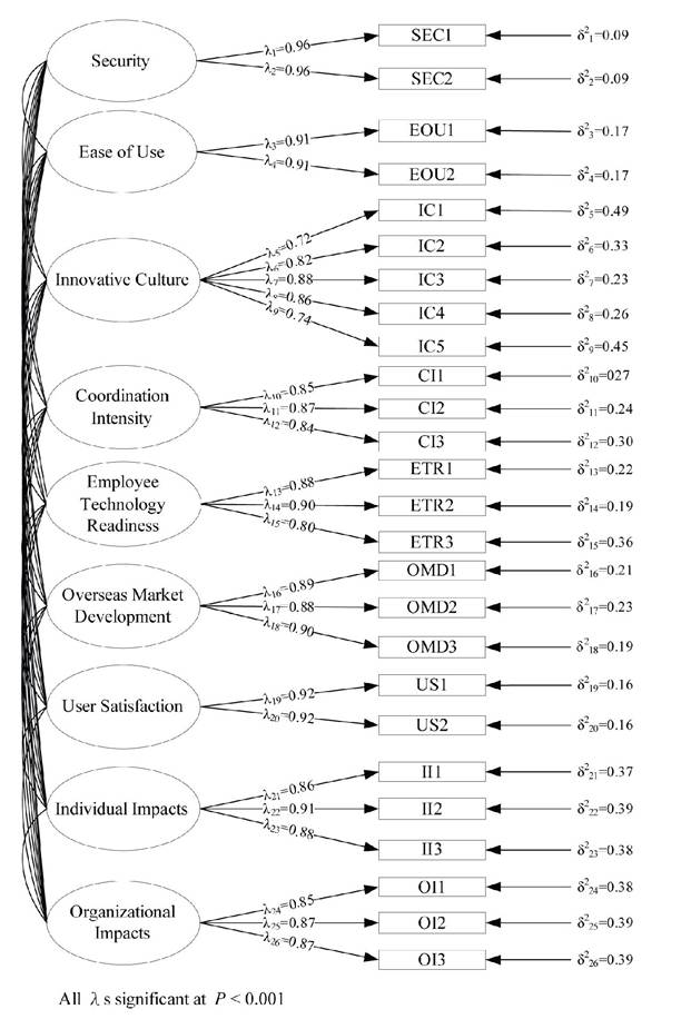
Fornell and Larcker (1981), indicating good converŁgent and discriminant validity of the measurement.
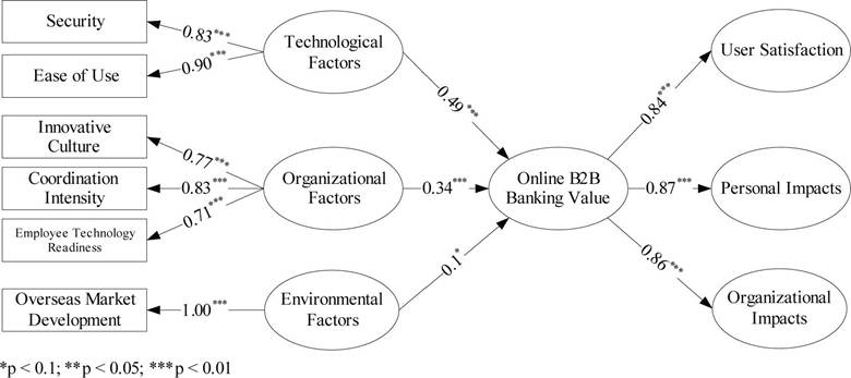
Structural Equation Modeling
Figure 3 shows a graphical representation of the structural model. The path coefficients, P-values, P-square, and t-values were examined in the staŁtistical model test in order to test hypotheses. The path coefficients are standardized regression coefŁficients and the P-values represent their respective significant level. P-square values refer to the total variance of dependent variable that can be explained by the path model. As shown, all coefficients are positive, indicating that as the value of independent latent variable increases, the value of the dependent latent variable also increases. Thus, as expected, these results support all hypotheses.
Table 3. Reliability, convergent validity, and discriminant validity
| Construct | CR | AVE | Shared Variance | ||||||||
| SEC | EOU | IC | CI | ETR | OMD | US | II | OI | |||
| SEC | 0.95 | 0.91 | (0.91) | ||||||||
| EOU | 0.90 | 0.83 | 0.26 | (0.83) | |||||||
| IC | 0.90 | 0.65 | 0.16 | 0.15 | (0.65) | ||||||
| CI | 0.89 | 0.73 | 0.08 | 0.17 | 0.12 | (0.73) | |||||
| ETR | 0.90 | 0.75 | 0.14 | 0.24 | 0.19 | 0.13 | (0.75) | ||||
| OMD | 0.92 | 0.79 | 0.12 | 0.15 | 0.03 | 0.10 | 0.07 | (0.79) | |||
| US | 0.91 | 0.84 | 0.34 | 0.43 | 0.17 | 0.22 | 0.20 | 0.18 | (0.84) | ||
| II | 0.91 | 0.78 | 0.19 | 0.29 | 0.16 | 0.12 | 0.32 | 0.12 | 0.32 | (0.78) | |
| OI | 0.90 | 0.74 | 0.16 | 0.36 | 0.16 | 0.09 | 0.26 | 0.07 | 0.30 | 0.51 | (0.74) |
Notes: CR = composite reliability; AVE = average variance extracted (also in parentheses).
Figure 3. Model testing results