3.4 MacArthur’s connection of LV to consumer-resource models
MacArthur’s (1970, 1972) consumer-resource system, described very briefly without equations in Section 2.2, features logistic resource growth and linear consumer functional responses.
MacArthur used the model to justify going back to the Lotka- Volterra model in some of his final work on the number of species that could coexist using a common set of logistically growing resources. It has continued to be used in theoretical analyses (e.g., Chesson 1990; Kuang and Chesson 2008). MacArthur implicitly assumed that resources never went extinct. However, a sufficient press perturbation to one consumer will often cause extinction or re-emergence of one or more resources. This is particularly likely when resources compete with each other (Abrams and Nakajima 2007; Abrams and Cortez 2015a). Hsu and Hubbell (1979) first identified the possibility of resource extinction, it was noted independently in Abrams (1980b), and its consequences for the relationship between the similarity in resource use and interspecific effects on abundance were explored in Abrams (1998, 2001a). However, the possibility of resource extinction has largely been ignored in the subsequent competition literature, even though it is a simple case of exclusion via apparent competition. This will be discussed again in Chapters 4, 5, and 6. Here I will just focus on how it changes the predictions of the LV model.A 2-resource version of MacArthur’s (1972) consumer-resource model is given by: 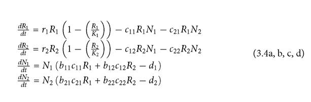 The only new parameter introduced here is the conversion efficiency of captured resource type j into numbers or biomass of consumer i, given by bij. An LV model (using the traditional form from Chapter 1) can be derived under MacArthur’s assumption of resources always at their quasi-equilibrium with respect to current consumer abundances.
Measuring competition: a consumer-resource framework • 43
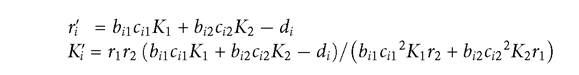
The two competition coefficients are given by:
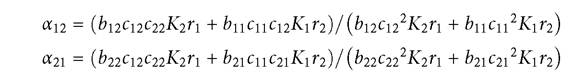
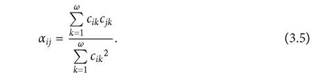
The above formulas are only valid provided that both resources have positive abundances at the equilibrium point. They simplify considerably if the resources are all characterized by equal values of the pairs of subscripted parameters K, r, and b. Under the equal parameter assumption, the formula for the competition coefficient can be generalized to the case of an arbitrary number of resources, giving the following formula for the effect of consumer j on consumer i relative to i on itself:
The sums here are over all ω resources in the system. In the case of two resources, if a consumer with significantly different consumption rate constants (c) on the two resources also has a sufficiently low mortality, one resource will go extinct when that consumer alone is present. Resource extinction can also happen in a 2-consumer-2- resource system, but this will imply extinction of one of the two consumers as well, given the above model. Ifboth resources persist at an equilibrium point, the two consumers must also have different relative consumption rates of at least one of the two resources to coexist for any range of mortality rates. In a multi-resource system, a sufficiently low mortality of either consumer may produce extinctions of one or more resources.
MacArthur also carried out some analyses that assumed an infinite number of resources that could be ordered using a single continuous variable. The attack rate of each consumer depended on that variable (here denoted x), which was usually exemplified by resource size.
He showed that if each species i had a Gaussian ci(x) curve having a different mean value, the competition coefficient was given by the analogue of eq. (3.5) with sums replaced by integrals over the variable x. Unfortunately, the weighting of different resources by b, K, and r was usually ignored in later work, despite an early article by Schoener (1974a), which stressed the large effects that these terms could have.Under the two-species LV model, the per capita effect of one species on the growth of another is independent of population sizes, and there is a linear reduction in each species' equilibrium abundance with increases in its own per capita death rate or decreases in the other consumer's per capita death rate. A sufficient change in mortality will result in exclusion of one species, but this happens continuously;
the equilibrium abundance of the disfavoured consumer species decreases linearly and continuously with increases in its mortality until abundance hits zero. Under MacArthur’s consumer-resource model, this remains true if all resources are present, but sufficiently large or small death rates may cause extinction of one or more of the resources. Because of the equal numbers of consumer species and resource types in the 2-consumer-2-resource system, extinction of one resource always results in extinction of one consumer (i.e., the one with a greater requirement for the single remaining resource).
Figure 3.1 illustrates a case in which either consumer (in the 2-consumer-2- resource system), if present alone, would cause extinction of one resource. Figure 3.1 assumes that the two otherwise similar consumers have opposite preferred resources. In the case illustrated, c12 = c21 = 1/4, and c11 = c22 = 3/4; each species consumes its ‘preferred’ resource at three times the rate of the non-preferred resource. I will later consider other parameter sets, but all are characterized by c11 = c22, and by cii + cij = 1.
In the figure, the two consumers have equal abundances when consumer 1 has a death rate equal to that of consumer 2 (d = 0.1). This basic equality combined with different resource utilization rates means that the two species are able to coexist for a range of values for consumer 1’s death rate. However, imposing a press perturbation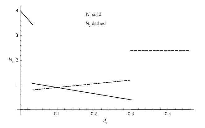
Fig. 3.1 Consumer populations as a function of the death rate of consumer 1 (d1) in a symmetrical 2-consumer-2-resource MacArthur system. The lines give the equilibrium abundances of consumer 2 (dashed) and consumer 1 (solid) as a function of the mortality of consumer species 1, d1. The other parameters are: bij = 1 for all i, j; d2 = 1/10; r = K = 1; c11 = c22 = 3/4. The extinction of consumer 1 at d1 = 3/10 corresponds to extinction of resource 2, while extinction of consumer 2 at d1 = 1/30 corresponds to extinction of resource 1.
to the per capita death rate of consumer 1 has the effects shown in the figure. Lowering consumer 1’s death rate causes an increase in its own density and a reduction in the abundance of consumer 2. However, with any continued directional change in species 1’s death rate, there is an abrupt loss of this equilibrium, at which point the system shifts to one having a single consumer and a single resource. If d1 is decreased to the point where consumer 2 and resource 1 go extinct, the result is an abrupt jump in the abundance of consumer 1. Note that this disappearance in Figure 3.1 occurs when the population of N2 is only approximately 11% lower than its equilibrium when both species have identical death rates and abundances. This extinction corresponds to a more than threefold jump in the abundance of consumer species 1.
The condition for such a discontinuous change in equilibrium abundance of a consumer species as the mortality rate of its competitor is reduced, is d < 2cii - 1 in a symmetrical 2-consumer-2 resource model with the other parameter values used in Figure 3.1.
For example, if cii = 3/4, as in the figure, a discontinuous change in the equilibrium of both consumers at a sufficiently low d1 occurs when the initial equal mortalities of both species are less than 1/2. Considering that a mortality rate of 1 implies extinction of either species, even in the absence of competition (given the other parameters assumed in the figure), species having mortalities much greater than 1/2 should be relatively unlikely to persist in a variable environment. This suggests that, if the model were a good description of the system dynamics, discontinuous responses to an altered mortality in one species should be quite common. There is a second discontinuity in Figure 3.1 if d1 is increased to a value of 3/10. This is characterized by the loss of both resource 2 and consumer 1, and by a discontinuous jump in the equilibrium density of consumer 2, which more than doubles its population size. Note that much of the literature in fisheries management is based on single-species logistic growth models. It suggests that reduction to half of the pre-fishery equilibrium abundance is a safe level of exploitation and is one that often produces close to the maximum sustainable yield. In this 2-consumer-2-resource system, the abrupt extinction of species 1 occurs when the added mortality to that species reduces it to slightly less than half of its original equilibrium.The model behaviour described above and illustrated in Figure 3.1 is unusual primarily in that the change in the mortality rate d of either species of consumer has a linear effect on equilibrium consumer abundances over some range of mortalities. In essentially all models other than MacArthur’s, the magnitudes of the population changes produced by a small press perturbation are quite sensitive to the initial equilibrium abundances of both consumers and resources (Abrams 1980b, 1983b). As a consequence, measures of the per capita effects of larger perturbations will depend on the initial densities and the magnitude of the imposed parameter change.
So far as I know, the phenomenon of discontinuous change illustrated in Figure 3.1 has not been demonstrated for the MacArthur model in any previously published work, although the possibility of resource extinction was discussed in Abrams (1998, 2001a). Given the long history of subsequent studies using or referring to MacArthur’s work, this figure demonstrates a lack of appreciation for the possibilities inherent in even this model that are inconsistent with the LV model.Adding one or two features that differ from MacArthur’s model gives rise to a range of additional phenomena. Figure 3.2 looks at the same type of mortality perturbation as in Figure 3.1. However, it plots one of the competition coefficients, α21, as a function of d1, rather than the abundances of the two species. It assumes a system that is similar to that explored in Figure 3.1 except that it has three resources, and the consumers have Holling type II functional responses, which saturate at high prey abundance (see Box 2.1). Each consumer utilizes one exclusive and one shared resource. The measure of competition given by expression (3.2) is calculated based
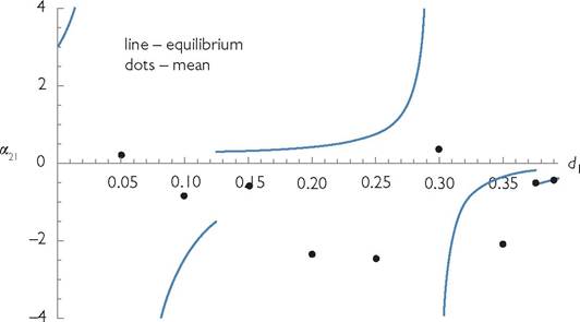
Fig. 3.2 Thelinesshowthecompetitioncoefficient (expression (3.2)) based on equilibrium densities (line segments) and mean densities (dots) for a system similar to eqs (3.4). This system differs in form from that in Figure 3.1; it has three resources rather than two; consumer 1 uses resources 1 and 2, while consumer 2 uses resources 2 and 3. It also differs in that the two consumer species have Holling type II functional responses with a common handling time for all consumer-resource pairs. See Chapter 6 for a more complete description of the model. The line gives the values of measure (3.2) calculated at the equilibrium point; both positive and negative effects occur. Most of the equilibria are unstable, and the dots give the analogue of measure (3.2) calculated based on change in long-term mean abundance following a 1% increase in the mortality rate from the value given on the x-axis. Positive values mean that the two consumer species change in the same direction in response to increased death rate of species 1; they change in opposite directions for negative values. The parameter values are: Ă1 = Ă2 = Ă3 = 2; K1 = K3 = 1; K2 = 2; c∏= 2/3; c12 = 1/3; c22 = 1/3; c23 = 2/3; bij = 1; d2 = 0.25. All handling times are hij = 2. This graph has four discontinuities corresponding to where a resource becomes extinct (d1 = 0.125 and 0.3928), and where a mortality of consumer 1 does not alter its density, at d1 = 0.05 and d1 = 0.2954. The system exhibits cycles at all of the mortality values when mean density effects were calculated, except for the two highest values.
Measuring competition: a consumer-resource framework • 47 on the equilibrium densities (solid line). For a selection of different initial mortality rates, the effect on mean densities due to a small finite change in mortality is given by the solid dots. Most parameters result in sustained population cycles and as a result the two measures (dots and line) differ significantly. There are pronounced changes in both measures as the mortality of one consumer is increased or decreased. Positive effects and very large magnitude effects are both possible. The figure illustrates the more general result that calculations based on an equilibrium point can be quite misleading as an indicator of the effects on average densities. As Chapter 6 will show, large-magnitude changes in measures of competition as neutral parameters are changed are common, even in systems that have relatively few differences from MacArthur’s model.
The remainder of this chapter will examine the structure and properties of consumer-resource models in greater detail, and will highlight how little we know about them, even in the case of a single consumer species. This implies that there exists a large unexplored frontier of different but biologically plausible models of competition involving two or more consumer species.
3.3