DIFFERENT FACETS OF INEQUALITY

There is much discussion ofinequality but there is also much confusion, as the term means different things to different people. Inequality arises in many spheres of human activity.

Even limiting attention to economic inequality, there are many interpretations and careful distinctions have to be drawn. It is convenient to first make a distinction between monetary and nonmonetary inequality. The former, refers to standard dollar-valued magnitudes associated with the economic activity of an individual or a household (earn­ings, income, consumption expenditures, and wealth). Nonmonetary inequality, also referred to here as “beyond income” inequality, addresses broader dimensions of eco­nomic life such as well-being or capability.

2.1 Monetary Inequality

Restricting inequality to monetary magnitudes does not prevent confusion. In the media, one often hears statements like “the wealth of the richest x billionaires would feed all the poor in a particular country.” But this confuses wealth, which is a stock, with income or consumption, which are flows. Flows have to be specified as occurring over a certain period, so that the figures for overall inequality in Figure 1a relate to annual income. Wealth, shown in Figure 1d, is in contrast measured at a point in time. If billionaires gave away all their wealth this year to feed poor families, then they would not appear in the Forbes list next year. If, on the other hand, they gave away the income from their wealth, then the gift would be smaller but they could go on doing it year after year.

There is often confusion between income and earnings. Articles in the academic lit­erature may contain in their titles the words “distribution of income,” but they are often actually about the distribution of earnings, and earnings are only part of income.

A person may have zero earnings, and no other income, but live in a household which is comfortably off. Such a situation does of course raise interesting questions—both for the analysis of inequality and in real life. What is the distribution within the household? The curve highlighted in the upper part of Figure 1a refers to the inequality of equivalized household income, which imputes to each member the total income of the household divided by the size of the household corrected by a factor that takes into account econ­omies of scale as well as age-dependent needs. This assumes that all household members enjoy the same well-being. The topic of intrahousehold inequality is addressed in Chapter 16 by Pierre-Andre Chiappori and Costas Meghir. As they stress, both the level of inequality and the trend over time may be quite different. This issue is particularly relevant to gender inequality, which is the subject of Chapter 12 by Dominique Meurs and Sophie Ponthieux.

Overall inequality is summarized in Figure 1 in terms of the Gini coefficient, and this is the statistic most commonly published by statistical agencies. The typical explanation of the coefficient is geometric: the Gini coefficient is equal to the ratio of the area between the Lorenz curve and the diagonal to the area of the whole triangle under the diagonal.

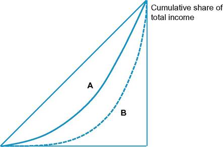
Cumulative share of total population

Figure 2 Lorenz curves. Note: The Gini coefficient of the distribution A is equal to the ratio to the whole triangle of the area between the curve A and the diagonal.

curves that do not cross, as with A and B, then one (in this case, A) definitely has a lower Gini coefficient. In this case we have Lorenz dominance, and A scores better than B on a wide variety of inequality measures (Atkinson, 1970). The converse is not true. The fact that the Gini coefficient is lower does not imply that the Lorenz curve is everywhere higher: the curves may intersect. The Gini coefficient can also be described in terms of the mean difference. A Gini coefficient of G percent means that, if we take any two households from the population at random, the expected difference is 2G percent times the mean. So that a rise in the Gini coefficient from 30% to 40% implies that the expected difference has gone up from 60% to 80% of the mean. Another useful way of thinking, suggested by Sen (1976), is in terms of “distributionally adjusted” national income, which with the Gini coefficient is (100G) percent of national income. So that a rise in the Gini coefficient from 30% to 40% is equivalent to reducing national income by 14% (i.e., (100 — 40)/(100 — 30) = 6/7 of its previous value).

We may be interested, not just in overall inequality, but also in the top and bottom of the distribution. The top income shares, for which we have the longest run of data in Figure 1, stretching back in the United States to 1913, show the share of total gross income (i.e., before deducting the taxes paid) accruing to the top 0.1%.

The panels in Figure 1 present therefore quite a rich picture of inequality in the United States over the past 100 years. But there is much that is missing. Figure 1 is a sequence of snapshots, rather than a movie. The top 0.1% in the United States in 1913 were those in the top group in that particular year; some of these people would have fallen out of the group by 1914. The statistics presented in Figure 1 tell us nothing about such mobility, which is the subject of Chapter 10 by MarkusJantti and Stephen Jenkins. As they explain, there are two aspects. First, there is the subject of how an indi­vidual’s income changes from one year to the next during their lifetime; on the other hand, there is the subject of income change between generations of parents and children.

Figure 1 shows evidence about the distribution of income within one country, but inequality is local and global as well as national. To begin with, money income has dif­ferent purchasing power depending on local prices, and geographical variation can have a significant impact, as has been shown in the work of Moretti (2013) on the college wage premium in the United States. Spatial inequality is highlighted by Ravi Kanbur in Chapter 20. As he notes, “the spatial dimension of inequality is a key concern in the pol­icy discourse, because it intersects with and interacts with disparities between subnational entities and jurisdictions. These entities sometimes have defined ethnic or linguistic char­acteristics, and in Federal structures have constitutional identities which naturally lead to a subnational perspective on national inequality.” Inequality equally intersects with con­cerns about globalization, which is the main subject of Chapter 20. The world distribu­tion of income is the subject of Chapter 11 by Sudhir Anand and Paul Segal—see also Bourguignon (2013).

We have referred above to the important topic of gender inequality. This is treated in Chapter 12, where the authors note that much of the literature is concerned with the gender gap in earnings. As they say, this is important, but only part of the story, since there is gender inequality in other forms of income and among those not in paid work, and all these inequalities interact with each other.

In introducing considerations such as gender and ethnicity, we are, however, going beyond straight income inequality as pictured in Figure 1. We are abandoning the ano­nymity that lies behind a Gini coefficient or a top 1% income share. We are asking how unequal income is across various well-identified groups. This is adding a dimension to the inequality concept. Two populations A and B may have the same overall inequality of earnings but the distribution of earnings may be exactly the same for men and women in A, whereas it may be more favorable to men in B. Two countries may have the same share of the top 1%, but in one country they may be all men. World poverty may have fallen, but the number in a particular ethnic group below the poverty line may have risen.

2.2 "Beyond Income" Inequality

Much of the reflection about inequality over the past 15 years or so has been concerned with extending the concept to “beyond income” inequality. As Sen et al. (2010) pro­posed to incorporate nonmarket dimensions into the measure of social progress, thus going “Beyond GDP,” the point here is also to take nonincome dimensions onboard when measuring inequality.

In addition to the quite remarkable perspective it offers on two centuries of economic thought on income distribution and redistribution, the chapter on the history of eco­nomic thought (Chapter 1) reminds us that there may be a historical bias in the way econ­omists see and think about income distribution and inequality. This bias is likely to be as present today as it was in the past. Classical economists focused on functional income distribution among land, labor, and capital because they viewed the society they were living in as made up of classes deriving their income from different factors. This view does not fit well our own world, even though factor rewards and the functional income distribution still features today in macroeconomic distribution theories. Another inter­esting feature of Chapter 1 is the long-lasting reliance in normative economics on util­itarianism. Itis only relatively recently, i.e., the 1970s, and very much under the influence of Rawls and Sen, which economists have begun to distance themselves from this approach and to consider alternatives.

It is noteworthy that this line of thought developed very much as a major extension of the previous literature on income inequality measurement, a literature that is compara­tively young in a historical perspective. Several features of the income inequality measurement “paradigm” as it developed say between 1920 (Pigou, 1920; Dalton, 1920)^[3] and the 1980s are worth stressing as it provides a point of reference for modern researchers who seek to extend this paradigm to a higher level of generality in terms of the definition of economic inequality. A first feature is that most properties of inequal­ity indicators, their interpretation in terms of social welfare, and their analogy with risk analysis are now well understood. To be sure, work remains to be done on the income inequality measurement agenda. This volume of the Handbook gives two examples of it: polarization (Chapter 5) and the introduction of statistical methods in the measurement of income inequality (Chapter 8 by Frank Cowell and Emmanuel Flachaire). But con­siderable progress has been made. A second feature is that this was done rather quickly after the contributions by Kolm (1966, 1971), Atkinson (1970), and Sen (1973). A third feature is that, despite a possible analogy with utilitarianism, the paradigm was explicitly presented as nonutilitarian, even in the generalized sense of a social welfare function, thus breaking with an important and powerful school of economic thought on social issues. Finally, as the paradigm started to develop, its very relevance was questioned. “Equality of what?” asked Sen (1980), suggesting that the income focus was severely restrictive and even questioning the welfare basis for inequality measurement.

Four chapters in this volume of the Handbook deal in different ways with this exten­sion of the income inequality measurement paradigm. The following simple framework is intended to help identify their main contribution, as well as the general issues in moving from income to other, more general, definitions of economic inequality. We first intro­duce the concept of “functionings,” in the sense of Sen, of individual i, denoted by the vector a_i. Functionings include various aspects of life enjoyment: material consumption, health, job market status, housing and environment quality, etc. Among them, let us sin­gle out material consumption, as measured by money income, y_i, so that a_i = (y_i,x_i) where x_i stands for nonmaterial consumption functionings. Let the preferences of individual i among those functionings be described by an ordinal utility u_i(y_i,x_i) function, normalized to unity for some reference bundle a°. Let the “satisfaction” of individual i be an increas­ing function S[u_i(y_i,x,), b_i] where b_i stands for a set of individual characteristics that can influence the satisfaction that individual i derives from (y_i,x_i). Finally, assume that the economic environment, the technology and social habits are such that the vector of func­tionings must belong to an individual-specific set Q_i defined by y_i, x_i, and z_i, where z_i is a vector of attributes of individual i, which may differ from b_i. A person may, for example, be able to function at home but not in a formal labor market setting or may come from a social background that broadens her economic opportunities. The set Q_i thus describes the set of functionings individual i can reach, given her characteristics. This may include the standard budget constraint as well as the production function that permits the

Introduction: Income Distribution Today xxvii

Introduction: Income Distribution Today

transformation into functionings of the goods and services bought on the market. Let (y*, x_i*) be the bundle of functionings preferred by individual i in the set of possibilities, Q_i. Of course both y* and x* are individual-specific functions of z_i. It is also natural to assume that this preferred vector is also the observed vector of functionings. The corre­sponding satisfaction of individual i is V_i = S[u_i(y*, x*), b_i], where the second argument allows for the fact that two individuals may get different levels of satisfaction from the same functioning bundles.

With the aid of this notation, it is then possible to describe the various approaches in the recent literature to extend the measurement of inequality beyond money income and to see their advantages and limitations.⁴ They are discussed in Chapter 2 by Koen Decancq, Marc Fleurbaey, and Eric Schokkaert on inequality and well-being, Chapter 3 by Rolf Aaberge and Andrea Brandolini on multidimensional inequality, and Chapter 4 by John Roemer and Alain Trannoy on inequality of opportunity.

2.2.1 Defining Inequality on Functionings: Multidimensional Inequality Measurement

Inequality is to be defined on the collection of vectors (y*, x*) in the population. Various approaches can then be used with varying degrees of generality. The most obvious way to proceed is to aggregate the various dimensions into a single scalar and apply standard uni­dimensional inequality measurement to this scalar. The aggregator function, defined as A(x,y), may be arbitrary, satisfying some basic properties, or it may be related to the framework set out in Section 2.2, in which case it is equivalent to assuming that all indi­viduals have the same preferences, u, and the same characteristics b, so that they have the same satisfaction function, S(u(x_i,y_i), b), of a functioning bundle (x_i,y_i). Alternatively, this function of (x_i,y_i) may be the preferences of the social evaluator. In any case, all individ­uals are assumed to apply the same trade-offs among the various functionings. Such a nor­mative aggregation approach lies behind several specific multidimensional inequality measures based on some functional form for the aggregator function, as in Maasoumi (1986). The new inequality-extended Human Development Index used in the Develop­ment Program of the United Nations (UNDP) (Foster et al., 2005; Alkire and Foster, 2010), or the recent efforts by OECD to measure multidimensional living standards tak­ing account ofinequality, unemployment, and health (OECD, 2014) are examples of this approach. The recent poverty measurement literature based on the counting of depriva­tions follows the same logic. Deprivations are grouped by functioning, then the number of deprivations and the extent of deprivation in the various functionings are aggregated to

⁴ It also allows us to distinguish the approach adopted in the inequality measurement literature of defining social welfare in terms of incomes y_i from an utilitarian approach where social welfare is defined over

generate an overall poverty indicator for individual i—see Alkire and Foster (2011) and Chapter 3.

Instead of using specific measures and specific aggregator functions, A(x,y) or S(u(x,y),b), it is possible to generalize social welfare dominance analysis in income inequality measurement—the counterpart to Lorenz dominance of income distributions (Kolm, 1977). Following Atkinson and Bourguignon (1982), a partial ordering of distri­butions of the bundles (y*, x*) in a population may be obtained by considering all the aggregator functions within some class of functions (see, for example, Duclos et al., 2011). As, however, is brought out in Chapter 3 by Aaberge and Brandolini, it is not straightforward to generalize the Pigou-Dalton principle of transfers to the multidimen­sional case. Moreover, we should not lose sight of the fact that nonmaterial functionings may require different treatment. The choice of aggregator function has to reflect the spe­cific characteristics of, say, health as a variable. For example, health may be measured in ordinal rather than cardinal form, as is discussed by Allison and Foster (2004) and Duclos and Echevin (2011).

2.2.1 Individual Preferences and the Income Equivalent Approach

Interpreted in terms of individual preferences, the preceding approach imposes identical preferences on all individuals. If ordinal preferences are observed, then a particular individual-specific aggregator function can be used which has the dimension of income—see chapter 4 of Fleurbaey and Blanchet (2013). With a reference vector x° of nonincome functionings, the equivalent income corresponding to an observed bundle (y_i,x_i) is given by the solution y_i of the equation: u_i(y_i, x°) = u_i(y_i, x_i). Such a solution does exist if u_i() is reasonably assumed to be continuous and monotonically increasing. The equivalent income is thus a function of the bundle (y_i,x_i) conditional on x°. It can be handled exactly in the same way as income is dealt with in income inequality measures. Of course, the issue is whether it is possible to estimate individual preferences u_i(y,x). In Decancq et al. (2014), this is done using subjective satisfaction data and relating these data to income and observed functionings for individuals with common characteristics in some subset of (b_i). Another issue is the choice of the reference nonincome bundle, x°, since inequality measures will be conditional on that bundle—see Chapter 2.

2.2.2 Defining Inequality Using Subjective Satisfaction

Going further along the chain, another approach at measuring inequality is to focus directly on satisfaction levels, V_i = S[u_i(y*,x*), b_i], as directly observed in satisfaction surveys. This is equivalent to using the individual-specific aggregator function, u_i(y_i*, x_i*), as well as the satisfaction function S(u,b_i). Several authors have followed this route, showing for instance that, unlike for observed income, inequality of “happiness” tended to go down over time in most developed countries and, as for income, to be smaller in richer than in poorer countries—see for instance Veenhoven (2005), Stevenson and Wolfers (2008) on the United States, Ovaska and Takashima (2010), Becchetti et al. (2011), and Clark et al. (2012).

Since life satisfaction is generally recorded on an ordinal scale, there are evident prob­lems in converting such measures to a cardinal scale and employing standard inequality indicators. For this reason, an alternative approach based on dominance criteria has been proposed by Dutta and Foster (2013). On the conceptual side, the issue arises as to the interpretation to be given to life satisfaction data. In particular, they may actually reveal the satisfaction of an individual relatively to his or her past experience and future expec­tations, and also possibly in relation to other individuals. If so they are improper for the measurement of “economic inequality.” In terms of the notation introduced above, it is doubtful whether the individual characteristics b_i, which determine how ordinal prefer­ences are cardinalized into satisfaction, should be taken into account in measuring eco­nomic inequality. The same bundle of functionings enjoyed by two individuals having the same preferences may yield different levels of satisfaction if one of them has a rather positive and the other a negative attitude toward life in general. A more detailed account of the interpretation to be given to subjective satisfaction data is offered in Chapter 13 by Andrew Clark and Conchita d’Ambrosio.

2.2.3 Inequality of Capabilities

Instead of defining inequality on the observed bundle of functionings (y*, x*), resulting from the choice of individual i in his/her choice set, Q_i, one could move upstream and consider the inequality of these choice sets, as in the capability approach. The first step is to identify these sets, as different from the particular point (y*, x*) actually achieved in the set. Presumably, this could be done by considering the set generated by all the function­ing bundles observed for persons with the same vector as attributes, z. Assuming that such identification has been made, the second step would consist of defining an inequality measure on these sets rather than scalars, as with income, or vectors as with multidimen­sional inequality. In practice, the measurement of inequality based on capabilities has been reduced to emphasizing a few components of the vector of individual characteris­tics, z_i, that indirectly define the size of the set Q_i. Typically, these are variables like education, health, or the availability of material resources. These three variables are com­bined linearly at the aggregate national level to define the familiar Human Development Index used by the UNDP to measure the inequality of functionings between any pair of countries. Several attempts have been made to incorporate a larger set of variables at the individual level in specific countries (see, for instance, Anand et al. (2007).

2.2.4 Inequality of Opportunities

Inequality of opportunity is defined as that part of the inequality in optimal functionings, (y*, x*), that is, due to differences in individual characteristics, z_i, or possibly in a subset of these variables. Among these characteristics, a distinction is made between variables, on the one hand, that are outside the control of individuals, which are called the “circumstances” faced by the individual, and variables, on the other hand, which may be assumed under his/her control. Then the inequality of opportunity can be measured by the inequality that exists in the (y,x) space across groups of people facing the same circumstances. Those groups are called “types” by Roemer (1998). The simplest measure is obtained by considering the inequality of the mean vector (y, x) among the various types. More elaborate measures would compare the distributions (y,x), rather than means, across types. In Chapter 4, Roemer and Trannoy discuss methods for doing so when focusing on income distribution only. The implementation of this approach requires assumptions to be made about what may be considered as “circumstances” (gender, eth­nicity, family background,...) and what may be assumed under the control of an indi­vidual (school achievement, for instance). Moreover, there are necessarily unobserved circumstances, so that one can at best measure the income inequality due to observed circumstances. A particular case frequently used is when one considers only one compo­nent of z_i, like ethnicity. In the space of earnings, the inequality of opportunity then cor­responds to the familiar concept of wage discrimination, as is discussed for gender in Chapter 12.

Inequality in terms of opportunity or capability is both defined on an “ex ante basis,” that is among groups of people with some common characteristics, and irrespective of differences in individual achievements in the space of functionings. (In contrast, inequal­ity of outcomes, be they income, earnings, consumption spending or even “satisfaction,” is an ex post inequality concept.) Practically, the main difference between the measure­ment of the inequality of capability and opportunity is that the former focuses on the inequality in the vectors of attributes, z_i, whereas the simplest approach to the latter con­siders the inequality between mean outcomes (y,x) across various “types” defined by identical “circumstances,” z. A second difference may lie in the individual characteristics selected to differentiate people, determinants of the set of possible functionings on the side of capabilities, and exclusively circumstances outside the control of individuals on the side of opportunity. Recently, there have been a number of attempts at measuring the inequality of opportunity in several countries—for instance, Brunori et al. (2013) have put together estimates obtained for a set of 40 countries using earnings as outcome and family background as circumstances. A related literature, although with more ante­cedents, is concerned with intergenerational income and more generally social mobility—see Chapter 10. Here too, the issue is to measure the contribution of an observed circumstance, the parents’ social status, the inequality of a particular function­ing, and the children’s social status.

Overall, “beyond income” inequality measurement touches upon the very funda­mentals of economic inequality and a number of important conceptual advances have been made since the pathbreaking work by Rawls and Sen. Data limitations, the frequent difficulty of translating conceptual parameters into actual figures, and quite often the complexity of the analytical instruments being proposed have limited the empirical appli­cations, but the area is promising for future research. A priority should be the search for simpler ways of making use of the conceptual advances in describing the multiple dimen­sions of economic inequality without reducing them to a single number.

3.