TAKING ECONOMIC THEORY SERIOUSLY

Data are one important ingredient in studying economic inequality; the second impor­tant ingredient is provided by economic theory, which underpins the search for expla­nations of inequality in Part III.

In this section, we focus on the determinants of market incomes: wages and capital incomes. These subjects, particularly wages, are covered extensively in other Handbooks, such as the Handbook of Labour Economics, and in designing this volume we have sought to avoid overlap. For the same reason, we have devoted more space to this aspect in this Introduction, as a contribution to bridge-building across fields of economics. We should also underline that while wages and the return to capital are important elements in deter­mining the distribution of household income, their impact depends on a variety of social and institutional mechanisms, such as household formation and demographics, and on the redistributive incidence of public policy (see Section 5).

4.1 The Race Between TechnologyZGlobalization and Education

In the Introduction to volume I, we set out the application of supply and demand analysis—perhaps the simplest of economic theories—to the explanation of rising earn­ings dispersion. Jan Tinbergen (1975) famously described a “race” between increased demand for educated workers and the expansion of the educated population. Where demand—driven by new technology or by globalization—outstrips supply, then the pre­mium for education rises. As typically portrayed, as in Figure 3, the supply and demand equilibrium is shifting up over time. The wage premium for higher-educated workers is rising because technological progress is biased in their favor—the skill-bias technical change (SBTC) hypothesis—or because increased global competition favors more

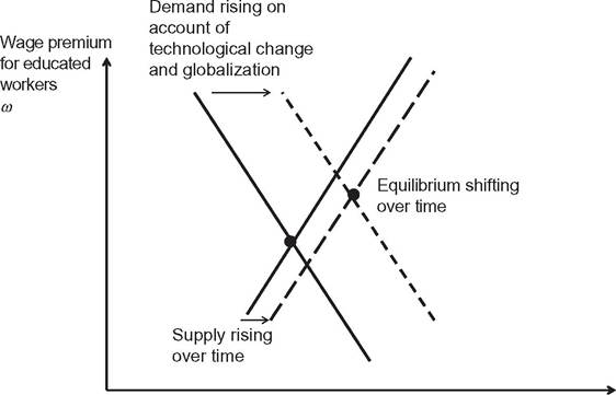
Ratio of higher-educated workers to basic-educated workers h Figure 3 The “race” between technology/globalization and education.

educated workers. In what follows, we refer mainly to the SBTC hypothesis, but this does not mean that we discount the role of international trade.

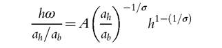
First year economics appears to explain what is observed in the real world. However, second year economics teaches us that a race is a dynamic process and its outcome depends on how one specifies the underlying adjustments. Suppose, as seems reasonable, that at any moment, t, the ratio of higher-educated to basic-educated workers is fixed at h(t) and that the relative wage, ω, clears the labor market. With aggregate output a function of the two kinds of labor, with a constant elasticity of substitution σ, the wage premium is determined by

where A is a constant and α_i denotes the productivity of workers of type i (h for higher- educated and b for basic-educated). If over time skill-biased technical change (SBTC) raises the square bracket, and if (a condition that is often forgotten) the elasticity σ is greater than 1, then the wage premium rises for any given h(t).

Suppose that the growth rate of h responds to the difference between the wage premium and the cost of acquiring education with an elasticity β; moreover, suppose that the cost of education, in terms of the wage of basic-educated workers, is equal to a fee, F, plus the cost ofpostponing earnings by Tyears, given by e^rl, where r is the annual cost ofborrowing, i.e.,

So that, combining (2) and (3)

and for positive ω the relative wage converges to a value

From this, we can see that SBTC (and σ > 1) does not lead to an ever-increasing wage premium. The move to a new, constant, rate of technological progress leads to an increase in wage dispersion but we should not expect this to continue, since supply adjusts.

We have set out this theory for two reasons. The first is that, when looking at the data, we need to distinguish between a continuing upward trend and an upward shift in the degree of wage dispersion. If, empirically, wage dispersion has ceased to increase, this does not mean that SBTC (or globalization) has come to an end.^[8] Indeed, from (5), we can see thatg falling to zero would imply that the wage premium fell back to its earlier value. The second reason for the explicit model of dynamics is that economic theory is valuable because it points to other mechanisms that may be important. From (5), we can see immediately that the same forces—SBTC or globalization—can have differing effects in different countries depending on the speed of adjustment of supply (via β).

4.2 Steady States and Transitional Dynamics

This condensed presentation of the supply and demand model of wage inequality shows the power of theory. At the same time, it raises questions as to whether the available models actually capture what is being observed and provide a reasonable basis for pro­jecting the future development and drawing policy implications. On the one hand, there is the issue of the relative strength of the various mechanisms simultaneously at play— e.g., biased technical change, educational choices, supply of skills, capital accumulation and allocation, etc. On the other hand, there is the issue of the time scale, which is a key aspect that we would like to highlight—both here and, later, when we discuss the dis­tribution of wealth.

To be tractable, the analysis generally focuses on the steady-state or long-run equi­librium properties of these models, without necessarily mentioning how long the long run is. In Chapter 14, Vincenzo Quadrini and Victor Rios-Rull thus warn the reader that: “for simplicity of exposition, we limit the analysis here to steady-state comparisons with the caveat that in the real economy, the distribution will take a long time to con­verge to a new steady state.” However, to bring theory to bear on the observed evolution of the distribution of income and on policy, tackling transitional phases is essential.

To illustrate this point, consider the dynamics of the preceding model in adjusting to a steady state, where again we focus on SBTC. This requires modeling with a little more detail the behavior of h, the ratio of the skilled, L_h, to the unskilled, L_b, labor force. Assume the population is stationary so that a proportion n of the labor force is exiting every year and an equal proportion is entering. For a stationary population, n would be the inverse of the duration of active life, roughly 2.5%. The important point is that most of the change in the skill structure of the labor force goes through its progressive renewal and modifying educational choices made by the entrants. More precisely, assume that the dynamics of the skill structure of the labor force is given by:

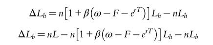
where L is the total labor force (L_h + L_b). In other words, the rate of growth of the skilled labor force depends on the net benefit from acquiring a skill from more schooling, whereas the growth of the unskilled labor force is driven by those entrants who have decided not to stay in school. Dividing these two equations respectively by L_h and L_b and subtracting the latter from the former yields:

which is a slight modification of (3).

Note that, with this modification of the labor supply dynamics, no steady state exists in the (2)-(3⁰) model as long as g is strictly positive. Simulating this dynamic system with σ = 1.2, h(0) = 3, n = 1/42, F = 1.9, r = 2.5%, T = 4, β = 1, and with no SBTC (g = 0%) yields an initial steady state. Then, in year 1, the rate of SBTC rises to g = 3%, and the economy evolves according to the trajectories shown in Figure 4 for the wage skill ratio or skill premium, ω, and for the size of the skilled labor force relatively to the number of unskilled workers, h. As before, the wage skill ratio rises, but—there being no steady state with positive g—it then falls back to the starting level.

Three features are of interest in Figure 4. The first is that, as expected, the wage skill ratio increases and then turns back down as the relative supply of skilled labor increases. Yet, this stabilization takes approximately 30 years to materialize. Even after 50 years, the curve has only just begun to turn down. The second feature is that the overall increase in the skill premium is rather modest, 3.1% in Figure 4. Such a limited increase is due of course to the labor supply response or the value of the elasticity β. Without such a response, the skill premium after 30 years of SBTC at the rate of 3% would have been 12% higher than initially. The third interesting feature in Figure 4 is the behavior of the skilled share of the labor force, which keeps increasing even when the wage skill premium has stabilized. In the presence of SBTC, such a persistent increase in the proportion of

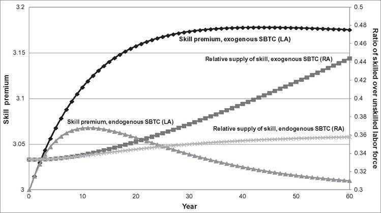
Figure 4 Skill-biased technical change: simulated trajectories of the skill premium and the relative supply of skilled labor with exogenous or endogenous rate of skill-biased technical progress. Note: The skill premium is shown on the left-hand axis; the relative supply of skilled workers on the right-hand axis.

skilled workers in the labor force is indeed needed to stabilize the wage skill premium and occurs because the long-run equilibrium premium is above the cost of acquiring a skill relatively to the unskilled wage level, unlike the case at the initial equilibrium.

Economic theory is thus important to understand switches from a long-run equilib­rium to another but also the nonsteady-state behavior. In this respect, note that the tran­sition modeled above depends on the way expectations are formed. Equation (3) and (30) are implicitly based on static expectations about the skill premium. Rational expectations are somewhat irrelevant in the present framework as the cause of the increase in the skill premium is not necessarily known by economic agents. But adaptive expectations might yield another time path. Likewise, a stronger supply response, β, to a change in the skill premium makes the transition shorter, and the new long-run wage skill ratio smaller.

From the point of view of the inequality of earnings, Figure 4 shows that two forces are at play. On the one hand, the increase in the wage differential increases inequality in the sense that the Lorenz curve shifts outward. On the other hand, the fact that more people get skilled has an ambiguous effect on the distribution of earnings. As the average earnings increases, both low-skill and high-skill people lose relatively to the average—the bottom of the Lorenz curve shifts outward but the opposite occurs at the top. The rela­tionship between these two ratios, ω and h, and the overall inequality as summarized by the Gini coefficient is discussed in Chapter 18. Note however, that this analysis refers to the distribution of earnings. Implications of the joint dynamics of technology and edu­cation for the inequality of income might be different because of various mechanisms including endogamy, joint labor force participation within couples or fertility differentials.

4.2 Endogenous Technological Change

To this point, technological change has been assumed to be exogenous, but the change in relative wages may induce a change in the degree of bias. In 1932, SirJohn Hicks rea­soned in his The Theory of Wages that “a change in the relative prices of the factors of production is itself a spur to invention, and to invention of a particular kind—directed to economizing the use of a factor that has become relatively expensive” (1932, pp. 124—125). This was later formalized in terms of the bias between capital- and labor-augmenting technological change by Kennedy (1964), Samuelson (1965), and Drandakis and Phelps (1965). More recently, it has been taken up in the form of “directed technical change” by Acemoglu (for example, 2002).

⁹ We may note that the induced technical progress literature identified the key role of the elasticity of substitution in determining the stability of the dynamic process governing the degree of bias: the condition for stability of the steady state in the model of Drandakis and Phelps (1965) is that the elasticity of substi­tution between capital and labor be less than 1. But the wage dispersion literature takes it for granted that the elasticity is greater than 1, which would be relevant if the same models were to be applied to the bias between skilled and unskilled workers.

Where technological progress is endogenous, this may substantially modify the tra­jectory of the economy. Following Acemoglu (2002), assume that the bias of technical progress is determined by the relative profitability of improving the productivity of the two factors of production. This profitability depends itself on two effects: a price effect, defined as the price of the technical bias—here the ratio ω∕(a_h/a_b)—and a market size effect according to which technical progress should favor the factor relatively the most abundant—i.e., the relative supply of skilled labor, h. Assuming that these two effects are multiplicative, and within the same CES framework as in (1), the relative profitability of investing in productivity gains of skilled labor thus depends on (Acemoglu, 2002, p. 790):

Then, the dynamics of the productivity differential can be specified as:

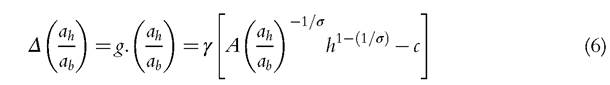
where c stands for the relative cost of developing technical progress in one factor in com­parison with the other and γ is the response rate of actual technical change to the eco­nomic incentive.

Adding Equation (6) to the preceding model (2)-(3⁰) modifies substantially the dynamics of the skill premium and relative labor supply. In the simulation shown in Figure 4, c is chosen so that (6) is initially stationary. Then an exogenous drop in the cost parameter, c, in year 1 triggers SBTC, initially at a rate identical to the exogenous rate, g, in the previous simulation (the response rate, γ, is taken to be 1). If the new trajectory is initially similar to the one obtained before, a divergence occurs after a few years. The rate of growth of the skill premium declines and a turning point is reached after 10 years. Then the skill premium starts falling as SBTC attenuates due to the negative price effect. If the relative supply of skilled labor keeps increasing—because the skill premium keeps being above its initial value—its rate of growth is much smaller than in the previous simulation. Interestingly enough, the new steady state to which the economy is very slowly converg­ing displays the same wage skill premium as initially, but a larger relative supply of skill. In other words, in the very long run the fact that the cost of improving the relative produc­tivity of skilled workers has fallen simply resulted in an increase in relatively more people being skilled. In the short run, however, the skill premium moved up.

This analysis demonstrates the value of theory in understanding the mechanisms behind the evolution of a simple aggregate inequality indicator like the wage skill pre­mium. It shows the need to consider transitional paths between equilibria, not just steady states, as well as the multiplicity of mechanisms influencing specific economic magnitudes to interpret their observed evolution.

4.3 Beyond Supply and Demand

The supply and demand story assumes that all agents act as price-takers: that we have perfect competition. As was observed by Michael Kalecki, “perfect competition—when its real nature, that of a handy model, is forgotten—becomes a dangerous myth” (1971, p. 3). In the real world, there are firms that have market power, as do collective organi­zations such as trade unions, and market power affects the operation of the labor market. The relative bargaining power of different actors determines the way in which economic rents are shared and hence the distribution of income. Power in turn is affected by the legal rights of workers, their representatives, and of employers. Such considerations turn the spotlight on governments, where the trend of recent decades has been to scale back the rights of workers, but also on employers. Where employers have market power, they can make choices regarding their employment practices, such as, for example, adopting the policy ofpaying “a living wage” or of limiting the range between top and bottom pay in their enterprise.

Bargaining power is not limited to firms and unions, as is shown by search and match­ing models of the labor market that involve individual workers and employers. Frictions in the labor market mean that, while ex ante competition may drive down the expected value of filling a job vacancy to the cost of its creation, ex post the matching ofa worker to a vacancy creates a positive surplus. Without a positive surplus, no jobs are created. The worker offered a job has a degree of bargaining power, since if he or she rejects the job offer, the employer has to return to the pool with the risk that no match can be secured. The magnitude of the risk, and hence the worker’s leverage, depends on the tightness of the overall labor market; the worker’s leverage also depends on the cost of remaining unemployed. The impact on the distribution of earnings depends on how bargaining power varies across jobs, but the important point is that market forces, even in a glob­alized world, impose only upper and lower limits on differentials. This becomes partic­ularly important when there are multiple possible market outcomes. Atkinson (2008) suggests a behavioral model of changing pay norms, where there is more than one locally stable equilibrium consistent with profit-maximizing behavior by employers. What has been observed in recent decades may be a shift from one equilibrium to another with much wider pay dispersion, particularly at the top.

There is therefore considerable scope for social institutions and social norms to influence the degree of pay dispersion, as is discussed in Chapters 18 and 19. In the latter, Forster and Toth note that “while it is widely recognized that institutions matter as an important factor for identifying the multiple causes of inequality... the weight attached to this factor in econometric studies has for a long time been limited” (p. 1801). As is stressed by Salverda and Checchi in Chapter 18, there is a pressing need to bring together the two rather separate literatures on supply/demand explanations and on institutions.

4.4 Bringing Back Capital

The SBTC explanation of rising wage dispersion focuses on the labor market, but—as the presence of the term e^rT in Equation (3) hints—we need to consider, not just the labor market, but also the capital market. Stated in terms of the aggregate production function, we have to consider not just F(L_b,L_h), where L_b denotes basic-educated labor and L_h denotes higher-educated labor, but F(K,L_b,L_h), where K is capital. We have to consider, not just the ratio of skilled to unskilled wages, but also the relative shares of wages and profits—the classical problem of distribution. Indeed, as in the classical analysis, we should extend the production function to include land and natural resources, N, giving output as F(K,L_b,L_h,N).

The extension to three, or more, factors means that substitutability and complemen­tarity becomes more complex, with richer potential outcomes for the distribution of income. The interesting possibilities include capital being a substitute for basic-educated workers but a complement to higher-educated workers. Such models, in the line of Krusell et al. (2000) are among those discussed in Chapter 14 by Quadrini and Rios-Rull. An alternative has been proposed by Summers in his Feldstein Lecture (2013). As Summers notes, capital can now be seen as playing two roles: not only directly via the first argument of the production function but also indirectly insofar as it supplants human labor through robotization. Denoting the first use of capital by K₁ and the second by K₂, the aggregate two-factor production function becomes F(K₁, AL + BK₂), where A and B depend on the level of technology. The production function is such that capital is always employed in the first use, but may or may not be used to supplement labor. The condition under which robots, or other forms of automation, are used to replace human labor depends, as one would expect, on the relative costs of labor and capital. Where there is perfect competi­tion, K₂ is zero where the ratio of the wage, w, to the rate of return, r, is less than A/B, and where K₂ is positive, then w/r=A/B. Theratio of the wage share to the capital share in the latter case is (A/B)/(K/L) and falls with the capital-labor ratio.

We can therefore tell a story of macroeconomic development where initially the Solow model applies: the capital stock is below the level at which w/r exceeds A/B. In this context, a rising capital-labor ratio leads to rising wages and a falling rate of return. The capital share rises if and only if the elasticity of substitution between capital and labor is greater than 1 (about which there is debate—see Acemoglu and Robinson, 2014, foot­note 12). Beyond a certain point, however, the wage/rate of return ratio reaches A/B, and K₂ begins to be positive. We then see further growth in the economy, as capital per head rises, but the wage/rate of return ratio remains unchanged. There is no longer any gain to wage-earners, since they are increasingly being replaced by robots/automation. What is more, the capital share rises, independently of the elasticity of substitution. It is as though the elasticity of substitution is increased discontinuously to infinity. In this way, the textbook Solow growth model can be modified in a simple way to highlight the central distributional dilemma: that the benefits from growth now increasingly accrue through rising profits. This outcome was indeed stressed some 50 years ago by James Meade in his Efficiency, equality and the ownership of property (1964), where he argued with considerable prescience that automation would lead to rising inequality.

4.6 The Distribution of Wealth

The distribution of wealth is the subject of the long-run studies in Chapter 7 by Roine and Waldenstrom and Chapter 15 by Piketty and Zucman. Both chapters show that the concentration of wealth was very high in the eighteenth to nineteenth centuries up until the First World War, dropped during the twentieth century, but has been rising again in the late twentieth and early twenty-first centuries. Chapter 15 shows that in France, the United Kingdom, and other countries, there has been a return of inheritance.

In Chapter 15, Piketty and Zucman begin by saying that

to properly analyze the concentration of wealth and its implications, it is critical to study top wealth shares jointly with the macroeconomic wealth/income and inheritance/wealth ratios. In so doing, this chapter attempts to build bridges between income distribution and macroeconomics.

Building such a bridge is indeed one of our aims in this Introduction, and, with this in mind, we return to the question of the timescale for the macroeconomic magnitudes. Denoting aggregate capital by w_t, aggregate income by y_t, and their ratio by β_t, we have:

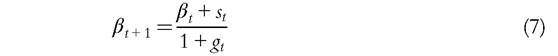
where s_t and g_t are respectively the net saving rate and the growth rate of income at time t. Assuming that those two rates are constant, the steady-state equilibrium of the economy is given by β* — s/g. With s equal to 10% and g equal to 3% per annum, the equilibrium capital-income ratio is 3.33. But, then, suppose that growth decelerates and the economy’s constant growth rate falls to 2%. The economy will then converge toward a new equilib­rium with a capital-income ratio equal now to 5. How long though will it take to get to this new equilibrium? As a matter of fact, the process described by (7) is quite slow. A simple simulation shows that, in going from 3.33 to 5, it will take almost 30 years for the capital­income ratio to reach 4, the double to reach 4.5 and more than a century to reach 4.8. As was shown many years ago by Ryuzo Sato (1963), the adjustment time in the neoclassical growth model can be extremely long. With such a transitional phase, relying on the steady-state properties of a theoretical model may be misleading for economic or policy analysis, even with a horizon of a decade. The direction of changes expected at equilibrium

¹⁰ As was pointed out by Sato (1966), the conclusions reached regarding convergence times are sensitive to the precise assumptions made concerning savings and technical change; the key issue is that transition path should be examined.

because of some exogenous modification or some policy changes is most likely to be felt along the whole transitional trajectory but their size might have to be substantially scaled down at the beginning of the transition. A tax on capital that reduces the saving rate by 1 percentage point, from 10% to 9%, for example, would lead to a drop in the steady-state capital-income ratio of 10%, but only 2.3% after 10 years and 4% after 20 years.

Let us now turn to the distribution of wealth. In that case, focusing on steady-states—or the golden rule—leads in some sense to the simple dismissal of distributional issues. Chapter 14 shows that any distribution of wealth combined with any distribution of work abilities is consistent with the steady-state equilibrium of the neoclassical model with dynastic agents, provided that aggregate wealth and aggregate effective labor satisfy some consistency relationship that involves the (common) rate of time preference of agents— the same kind of result holds trivially in endogenous growth models of the AK type, see Bertola et al. (2006, chapter 3). This is fine but possibly of limited practical relevance. Assume indeed that an economy initially at a steady state with a distribution D of wealth is then subject to some shock, for example, a technological shock or an income tax, that modifies its aggregate long-run equilibrium. Then, in moving toward this new equilib­rium, the distribution D will change and, at the new equilibrium, there will be a new distribution D⁰. The fact that this new aggregate equilibrium may be supported by another distribution than D⁰ is not the relevant point. What we are interested in is the change from D to D⁰ and this is certainly not indeterminate. Likewise, the indeterminacy of distribution in a steady state does not mean that redistribution has no macroeconomic effect and no impact on the primary distribution of income. As long as redistribution can­not be lump sum, it will modify both the steady-state equilibrium and the distribution of primary and disposable income.

The models in Chapter 15 of the distribution of wealth are rather different and have different long-run properties. The treatment of time is again important. To be precise, let us take the unit of time as the lifetime (identical for all), with the present value of inherited wealth of individual i denoted by w_i∙_t. It is assumed that lifetime savings are a constant proportion of the aggregate of wealth and income:

where y_Lt is the lifetime labor income, assumed to be identical across individuals, R is the rate of return over the lifetime, and S_it, the individual saving rate defined on wealth plus lifetime income. S_it is assumed to be independently and identically randomly distributed around some mean value, S, across periods. Aggregating the accumulation equation over all individuals in a generation yields:

Combining (8) and (9) and assuming that the aggregate economy has converged to a steady state, it is shown in Chapter 15 that the dynamic behavior of the wealth of

individual i, relatively to the mean wealth of the population, z_it, is given by the following multiplicative stochastic difference equation:

where G is the rate of growth over a lifetime.¹¹ Under the condition that φ < 1, the steady-state stochastic distribution of z_it has a Pareto upper tail, with a Pareto coefficient that decreases with φ, where a smaller coefficient corresponds to greater concentration of wealth. Denoting the annual rate of interest by r and the annual rate of growth by g, and assuming a lifetime of H years, φ can be expressed asIt follows that long-run

wealth concentration increases with r—g; it is also clear that concentration increases with the savings rate, S. Both elements have a role to play.

Suppose, instead, that one adopts an intragenerational perspective, with the time unit as the year rather than a lifetime, and assumes that people save a proportion of their current income, s_it, drawn randomly from some distribution with expected value s. Then (8) and (9) are transformed into:

where y_t is now the common annual wage income. Assuming a steady state with growth rate, g, and using the same kind of derivation as above, the stochastic difference equa­tion (10) becomes¹²

Under the assumption that E(rs/(1 + g))(s_it/s) + (1/(1 + g)) < 1 or rs id="Picutre 25" class="lazyload" data-src="/files/uch_group77/uch_pgroup315/uch_uch7351/image/image025.jpg">

This implies:

and then plugging that expression back into (13) leads to (12).

Pareto coefficient that decreases, and a wealth concentration that increases, with rs∕(1 +g). This refers to the distribution of current wealth, since there is a fresh drawing of s_it each period of life. (The independence assumption has therefore quite different implications.) In this model, it is the balance between rs and g that determines the long-run distribution, as in the early models of Meade (1964) and in the primogeniture version of Stiglitz (1969).^[13]

Which model is the most appropriate? With the long horizon adopted to study the evolution of the distribution of income and wealth in Chapters 7 and 15, it would seem that the intergenerational framework is the most appropriate. It can also be argued that the assumption about randomness, with persistent lifetime good or bad luck, captures better our distributional concerns. Against this, it is the distribution of current wealth that is observed (as, for example, in Figure 1). It has, however, been shown by Benhabib, Bisin, and Zhu that when a model of lifetime wealth accumulation, with a realization fixed for any household during its lifetime, is embedded in a model of the current dis­tribution of wealth, then “the power tail of the stationary distribution of wealth in the population is as thick as the thickest tail across the wealth distribution by age” (2011, p. 132). Put loosely, the upper tail of the current distribution tends to be dominated by the most unequal generation. But, it remains the case that the full effect of an increase in r—g from today onward is bound to be observed only some generations from now. As a matter of fact, the inegalitarian effect that will be observed in the second or even third generation might be very limited and r—g may change again in the distant future.

The conclusions that we draw are twofold. The first is that, as in the discussion of mobility in Chapter 10, it is necessary to consider both the intra- and the intergenera- tional dimensions, and that in both cases a better understanding of the transitional periods seems crucial. The second is that the evolution of the distribution of wealth depends on savings behavior, on the rate of return, and on the rate of growth. In this context, we should not forget that there were two arms to Kuznets (1955) Presidential Address, in which he sought to explain why inequality was at that time falling despite the existence of long-term forces leading to higher inequality. One arm was the theory of structural change that has come to characterize his approach, but the other was the concentration of savings in the upper income groups. This led him to conclude that “the basic factor militating against the rise in upper income shares that would be produced by the cumu­lative effects of concentration of savings, is the dynamism of a growing and free economic society” (1955, p. 11).

5.