THE RESEARCH QUESTION AND METHODS TO EXPLAIN INEQUALITY AND ITS CHANGE

This chapter sets out the problem of a multicausal explanation of income inequality in a cross-country context. First we present the structure of the problem and then we provide an outline of the methods used in the literature we review.

19.2.1 The Structure of the Research Question

To understand and place the formulation of the research questions of the literature, it is useful to start with a very general flow chart showing the major elements of inequality formation (see Figure 19.1); this deliberately ignores potential causality directions at this stage. As the figure illustrates, income inequality (at all levels of economic development) is a product of macro processes (such as supply and demand processes, globalization, trade,

² However, these selection criteria could not always be fully respected. For example, the data background of certain studies we reviewed seemed at first glance to not properly fit the above criteria, for example, when a model of an important political process (such as corporatist agreements) is tested with individual wages rather than incomes. However, the line of argument dealing with the political economy of interest groups remains of interest even if it refers to the effect on wages only. Also, in some cases, especially in the frame of the debate on globalization and technological change, lessons from developing countries may be impor­tant for theoretical or methodological reasons, so some of those studies with coverage of countries outside of our prime target have not been excluded. The general guidelines from the above limitations, however, remain to be held.

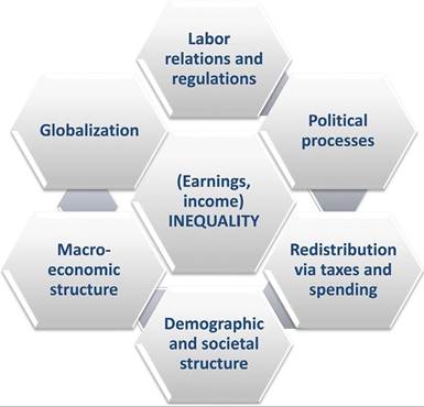
Figure 19.1 Stylized description of determinants of income distribution.

and sectoral change in the economy); structural conditions (in terms of economic and social structures as well); and institutional constructs (political institutions for the aggre­gation of collective preferences, labor market institutions to assist an efficient utilization of human capital endowments, and tax/transfer schemes for institutionalizing redistribu­tion in society).

Schematically, Figure 19.1 numerates six families of potential key drivers of earnings and income distributions. From left to right, “globalization” is primarily meant to cover the economic dimensions of globalization, such as increased trade integration, outsour­cing or financial integration. Technological changes also fall into this family. Next, under the heading “labor relations and regulations,” we also discuss institutional features of the labor markets, such as the level of unionization, the potential role of wage-bargaining institutions, or levels of corporatism embedded into the political system. “Political processes” include preference formation (of voters and of parties), political representa­tion, and interest group politics. “Redistribution and tax-transfer policies” involve var­ious policy arrangements aimed at altering the “original” distribution that came about as a result of market processes. “Demographic and societal structure” refers to the way indi­viduals (with their own incomes) combine into families and households (household structure by age, employment, income levels) and how the society is composed of various sociodemographic variables (such as age, gender or education). Finally, the “macro­economic structure” of societies (characterized by sector distribution of employment, by degrees of labor market attachment, etc.) is of central importance for the determina­tion of overall inequalities. With this schematic we illustrate the complexity of factors that affect income distribution and highlight the partial nature of most empirical analyses we found in our literature search.^[254]

The overwhelming majority of the articles we reviewed model inequality (or inequal­ity changes) and regress a chosen inequality measure on selected driver variables, usually among one (rarely more) of the driver families. Among this literature, the list of 48 articles with key features analyzed and that come closest to satisfying the criteria above can be found in Annex Table A19.1.

A general formulation of the approach taken can be written in the form of a gener­alized regression equation (Equation 19.1).

where INEQ_{i t} is a properly chosen measure of inequality of household incomes within country i at a certain point in time t, and X_it = {x,∙_it} is the vector of population char­acteristics aggregated from individual (or household) attributes (age, education, sex, household type, etc.). On country level these attributes define the structural conditions to inequality development in a certain country.is the vector of macroeco­

nomic (GDP, trade, financial globalization, technology, etc.) and institutional variables (policies, redistribution, wage-setting mechanisms, etc.). In a cross-country comparison, where the unit of analysis is country, these variables enter as attributes of the macro units (countries); Q_it = {qjj_t} is the vector of specific historic/contextual variables (history, size location, composition, etc). η_i And μ_t stand for the inclusion of country and time dummies, respectively (these occasionally entail, as fixed effects, a large variety of country-specific attributes and year-specific effects). ε_it Represents the error term, i is 1, ∙ ∙ ∙, N for countries, and t is 1, ∙ ∙ ∙, T for years. Forlateruse we denote Equation (19.1) as a grand inequality regression equation (GIRE).^[255]

19.2.2 Notes on the Arguments and Parts of the Grand Inequality Regression Equation (GIRE)

Atkinson and Brandolini (2009) advise readers hoping to understand the empirical inequality literature that they should consider theory, data and estimation together, meaning that data have to be sufficient and adequate to theory, and estimation methods have to be adequate to available data.

19.2.2.1 The Usefulness of the General Formulation

An important point concerning the regression approach should be addressed at the outset. Some scholars may argue that cross-country regressions fail to capture adequately the cross-country differences because historical and institutional specificities define completely different relationships between dependent and independent variables. Others argue that the relationship between variable X and variable Y will be the same when con­trolled for all other potential factors. We think that well-specified regressions can help in understanding links (even if not causalities) between various factors, but, at the same time, caution is warranted, and country specificities always have to be taken into account. Clas­sifications of various welfare regimes (going back to the seminal work of Esping­Andersen, 1990, differentiating between the conservative, the liberal and the socialist regimes) or differentiations between such complex settings as varieties of capitalism (Hall and Soskice, 2001) can add important parameters, and they do describe different sets of circumstances, but controlling for them (in an ideal data case) leaves sufficient room for the relationship between X and Y to operate uniformly across countries.

Taking—admittedly—to the extreme the welfare regime literature, however, makes it quite difficult to identify the contribution of the various single factors to income dis­tribution (or a change in it). Given that welfare regimes are defined as a complex interplay and a joint product of the state, the market and the family (Esping-Andersen, 1990; Esping-Andersen and Myles, 2009), the proper methodological analogy would be cluster analysis rather than regression. Clusters built from a wide array of country attributes could show similar and dissimilar country examples of inequality, together with the other observed factors (Kammer et al., 2012 is a prominent example of this type of analysis of welfare regimes).

⁵In fields where institutional complexities of the subject and the training background of scholars induce widespread use of qualitative methods, an explicit mention of this caveat is important (see, for example, Rueda and Pontusson, 2000 warning for political scientists or Kenworthy, 2007 message to sociologists).

19.2.2.2 The Units of Analysis

In cross-country explanations of inequality drivers, the units of analysis (data points) are countries, characterized by various inequality measures as left-hand variables and other macro characteristics such as GDP, shares of economic sectors, globalization, institutions or redistribution as right-hand variables. In most of these analytic attempts a time dimen­sion is introduced on the right-hand side with the use of multiple data points for various periods. This in some cases allows for a macro-level analysis of changes.⁶ Many reviewed studies belong to this class. It would, however, be ideal to have analyses of pooled micro­data to identify cross-country differences of determinants of income inequality. Surpris­ingly enough, we did not find articles that fit into the latter category.

Another strand of analysis, again using micro rather than macro variables to explain the underlying drivers of inequality (and of changes in inequality), makes use of decom­position methods. Decomposition can be a powerful instrument to disentangle mathe­matically the different components that make up overall inequality. Decomposition can be used to identify the relative roles of several income sources to overall income inequal­ity (tracing back to Shorrocks, 1982) or else to analyze the contribution of different pop­ulation subgroups to levels of and trends in inequality.

19.2.2.3 Regression Methodology

The majority of macroeconomic cross-country panel studies reviewed use ordinary least square (OLS) regression with pooled cross sections in a macroeconomic setting to gauge causal factors impeding between- and within-country inequality.

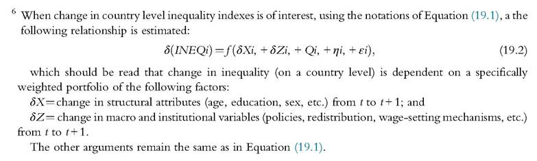
differ across countries. Both patterns would lead to inefficient OLS estimates if not treated properly.

To assign country-specific factors to country-specific intercepts rather than constrain­ing all countries to the same intercept, a large majority of the macroeconomic panel approaches reviewed here apply fixed effects in their models. Gourdon et al. (2008), for instance, put forward as one of their main conclusions that “results from studies that do not control for effects of omitted variables via fixed effects are biased” (p. 352).

However, some authors consider fixed-effects methodology overly conservative because any variation between countries is disregarded in the data and the effect of some factors that are constant over time but differ between countries, such as institutions, are likely to be overlooked. This is the line of argument of, for example, Nielsen and Alderson (1995) and Alderson and Nielsen (2002), who propose as an alternative a random effects model (“random” in the sense that it treats unobserved effects as random variables because they are treated independent of the explanatory variables). Such a model removes only a fraction of the country-specific means, not the whole mean, and is thus considered as “less wasteful of between-country variation” (Alderson and Nielsen, 2002, p. 26).

There also has been more general criticism of the usefulness of time series regression methodology for explaining inequality determinants. One issue is that of identifying long-running relationships and cointegration of series. A problem with the standard panel regression approach is how to account for the timing of the effect of the explanatory vari­ables. Globalization or deregulation, for instance, may well be “significant” factors but they may take some time to affect the distribution; furthermore, the delay may not be the same across countries and across factors. This may be less of a problem if long-enough time series were available, but this is generally not the case.

A related issue is that of the nonstationarity of data points, that is, that they have means and variances that change over time, either in trends, cycles or at random. Parker (2000), for instance, argues that the fact that many explanatory variables are likely to be nonsta- tionary produces spurious regression results in that they may indicate a relationship between two variables where there is none. Further, the power of integration and coin­tegration tests tends to be low when small sample sizes are used, which is often the case in studies of inequality.^[256] One possible solution is to combine OLS with the method of error correction models proposed by Hox (2002) and applied, for instance, by Rohrbach (2009) or Cassette et al. (2012). This method regresses the lowest-level variable on cov­ariates from all other levels simultaneously.

Similarly, Jantti and Jenkins (2010) argue that direct estimation of parameters in time series analysis can be problematic because of the nonstationarity of both left- and

right-hand variables. Further, left-hand variables are typically bounded, usually to the unit interval, which involves problems for tests of stationarity and also raises more general issues about the appropriate specification.⁸ Jantti andJenkins (2010) propose returning to parametric distribution functions instead. Applying the latter approach to UK data, they found a lesser distributive effect of macroeconomic factors than is suggested when com­monly used methods are applied.

That said, even if cross-country panel regressions entail a number of interpretational problems and often, taken together, provide inconclusive findings, especially with regard to the role of globalization, much has been learned from the studies undertaken during the past decades. As Eberhardt and Teal (2009) put it (referring to controversial findings of cross-country growth regressions), “the lesson of incomplete success is not to abandon the “quest” but to seek to understand why success has been so limited” (p. 28).

The most common approach to explaining changes in inequality in the studies reviewed is with aggregate inequality measures. By doing so, however, one might miss important changes in the distribution. From that point of view, it may be worth pursuing more comprehensive approaches, such as the reweighting procedure proposed by DiNardo et al. (1996), as well as the recentered influence function regressions by Firpo et al. (2009) for labor market analyses or the microeconometric approach by Bourguignon et al. (2005) to the household income distribution in the microeconomics of income distribution dynamics project. All these approaches aim to shed light on the drivers behind changing income distributions by simulating counterfactual distributions in a controlled manner.

Such approaches remain on a partial equilibrium view. Another challenge today, therefore, is to bring together macro- and micro-based regression methodologies and their findings. To that aim, new tools of macro-micro models have been developed (see Bourguignon et al., 2010). These models analyze, for example, the distributive effect of “macro” events, such as migration, by integrating a macro framework with a micro­simulation model that uses household or individual data, either by implementing a sequential approach (e.g., first computing the macroeconomic variables in a computable general equilibrium model and then using estimated values as input for a microsimulation model that distributes the effects of macro changes among micro units), or via full inte­gration of microsimulation models within computable general equilibrium models.

In terms of the presentation of results from cross-country panel regression studies, in addition to indicating the significance of coefficients, many studies try to gauge the relative importance of the different variables that have been estimated to affect inequality. Because the variables under examination often are measured in different units, a common approach is to calculate standardised coefficients (which are obtained by first

Following Atkinson et al. (1989,p. 324-325), there is a case for using alog-logistic formulation of the type log[INEQ∕(1 — INEQ)], which allows unbounded variation.

standardizing all variables to have a mean of 0 and a standard deviation of 1). Moreover, simple simulations or a back-of-the-envelope calculation often are used to quantify the effect of an individual factor. For instance, IMF (2007) and Jaumotte et al. (2008) calcu­lated the contributions of various factors to the change in inequality as the annual average change in the respective variable multiplied by the corresponding coefficient, and the averages across country groups were weighted by the number of years available for each country (to increase the weight of countries with longer observation periods in these averages). The OECD (2011) makes use of the same computation approach to show the relative size of the contributions of different factors to the increase in overall earnings inequality.

19.3.