Possible World Semantics for FOLP
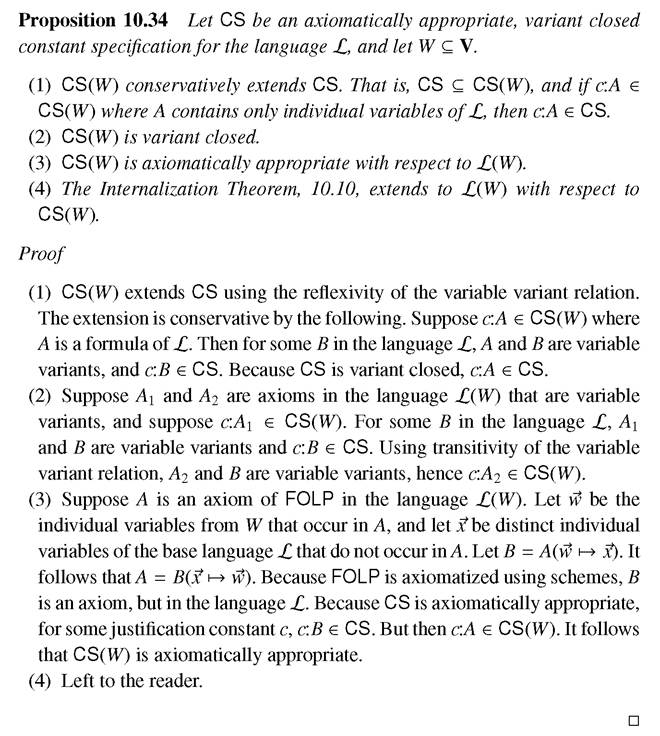
Starting in Section 10.4 an arithmetic semantics is presented for FOLP—an essential step for an arithmetic interpretation of quantified intuitionistic logic. Of course this is closely related to the material found in Chapter 9.
But first, in this section, a possible world semantics is given, combining features of first- order Kripke models for S4 with features of the possible world semantics for propositional justification logic given in Chapter 4.10.3.1 The Ideas Informally
Fitting models for propositional justification logics are built on top of propositional Kripke models. In a similar way first-order justification models are based on the possible world semantics appropriate for quantified modal logics. Because we want a justification analog of first-order S4, we build on possible world frames having a transitive, reflexive accessibility relation. The most common first-order S4 models also have domains of quantification associated with each possible world, meeting a monotonicity condition. Monotonicity says that if possible world A is accessible from possible world Γ, then the quantification domain associated with Γ is a subset of that associated with A. Why monotonicity? As was the case historically with LP, the ultimate goal is to provide a semantics for intuitionistic logic, though now quantifiers are involved. But why should intuitionistic logic have something to do with monotonicity?
Classical mathematics is Platonic—its structures are simply there, changeless and timeless. Many mathematicians think they are discovered and not created. Constructive mathematics is decidedly otherwise. Brouwer talked about the creative subject, who actually constructs mathematical objects. Free choice in the process is allowed. In fact, these ideas are not really foreign to the classical mathematician. Mathematical structures that are not known to us are as if they aren't there at all.
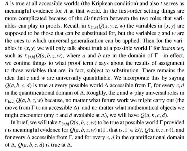
At one time there were no such things as complex numbers within the known mathematical universe. Historically, they gradually moved into our view. Whether they were there all along is not epistemically important. What is important is that, in the realm of what we know, complex numbers once were not, and then were. It is reasonable to assume that after creation as in intuitionism, or discovery as in Platonism, a mathematical structure continues to exist, or to be known. We do not forget. Whether we consider things constructively or epistemically, monotonicity and not constant domains is appropriate.Propositional connectives will be truth functional at each world. Quantification at each possible world is over the domain associated with that world. The central issue is how proof terms, or justification terms, behave. As an example we consider the formula ) at possible world Γ. In this formula
occurrences of x and ó are free, but not those of z or w. We could use the machinery of valuations to assign values to free variables, but it is simpler and more perspicuous to allow members of domains to appear directly in formulas. Say a and b are in the quantification domain associated with Γ; we will talk about instead of talking about
 under the val
uation that maps x to a and ó to b. With this notational convention understood, what should it mean for to be true at Γ? Much as was the
case with propositional justification logics, there will be two conditions, one syntactic, one semantic.
We use the evidence function machinery we have already seen in the propositional setting, Section 4.2.
Recall that for an evidence function E, for each proof term t and each formula A, E(t, A) is the set of possible worlds at which t can serve as meaningful evidence for A. Of course E must meet certain closure conditions, and this will be taken care of in Definition 10.21.In propositional Fitting models we take t:A to be true at a possible world if
10.3.2 FOLP Fitting Models
We begin with a small word about terminology. In Definition 10.6 FOLP0 was characterized axiomatically, then FOLP was introduced as FOLP0 combined with the total constant specification. Here we will be a little more nuanced in our requirements for constant specifications, and so we will write FOLP(CS)
The following formal definitions incorporate, quite directly, what we discussed informally in the previous section.
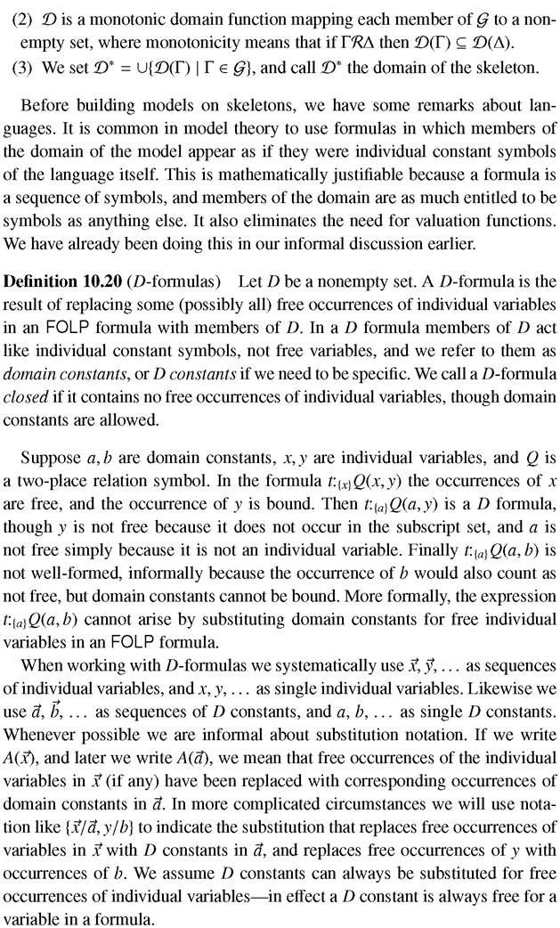
Definition 10.19 (Skeleton) 1
1 

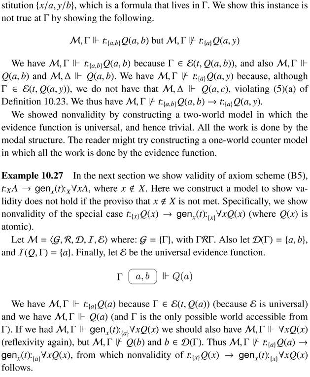
A [a, b, IF Q(α, b)
Consider the instance of t{xy Q(x; y) → tf xg Q(x; y) resulting from the sub
10.3.4 Soundness
Axiomatic soundness follows the standard pattern. We omit explicit discussion of constant specifications, which is straightforward.
Each of the FOLP0 axioms is valid in all Fitting FOLP models, the rules preserve validity, and hence each theorem of FOLP0 is valid. We show this for four representative axioms and omit discussion of the rest, and to keep notation simple we work with special cases that are sufficiently typical. In what follows, assume is a Fitting FOLP(CS) model.
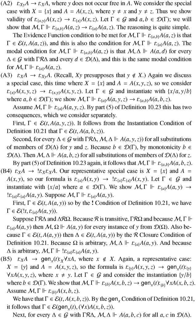
The other axioms are valid, and the rules preserve validity—verification is left to the reader. It follows that the axiom system for FOLP0 is sound with respect to the Fitting semantics. Further, constant specifications are quite straightforward and are left to the reader.
Theorem 10.28 (Soundness) Let CS be a constant specification. Ifthe FOLP formula A is provable using constant specification CS then A is valid in every Fitting FOLP(CS) model.
10.3.5 Language Extensions
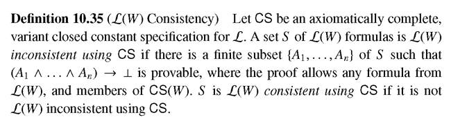
Constant specifications require some care. In the propositional setting soundness holds with respect to any constant specification, and we saw in Section 10.3.4 that this carries over to FOLP. Propositionally, for completeness, we had to require the condition of axiomatic appropriateness for constant specifications, Definition 2.7. Not surprisingly this is also the case when quantifiers are involved. The following is a version appropriate to the present setting.
Definition 10.30 (Axiomatically Appropriate) A constant specification CS is axiomatically appropriate if, for every axiom A, there is a proof constant c such that c:A ş CS.
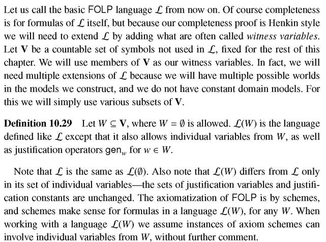
Our central problem with justification constants is how to extend constant specifications from the base language L to the various languages L(W) that we will need in our model construction.
We could, of course, simply work with universal constant specifications, but that is actually more stringent than we need. Instead we will require that constant specifications for L meet a condition that amounts to saying it is the pattern of individual variable usage that matters, and not what we call particular variables. This is a reasonable requirement that behaves well with respect to language extensions. The universal constant specification meets this condition, but so do others.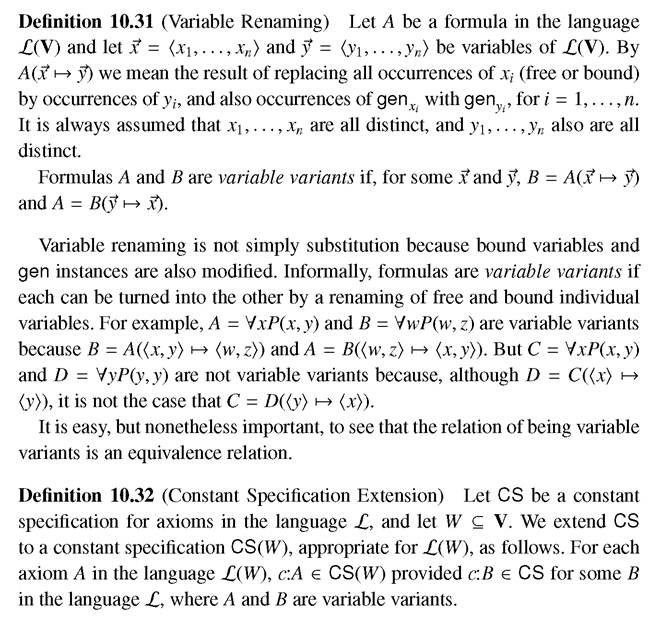
Constant specification extensions behave nicely provided we impose the following condition.
Note that W can be 0, so the preceding definition also specifies what it means for CS to be variant closed for L. Here is what we meant when we noted that variant closure entailed nice behavior.
10.3.6 The Canonical Fitting Model
In this section we construct a kind of canonical model, and then use it to prove completeness in the following section. Completeness is for formulas in the language L, using a constant specification CS that is axiomatically complete and variant closed. The construction is Henkin style. Possible worlds are, essentially, maximally consistent sets of formulas whose domains contain witnesses for the true existential formulas. Providing for the existence of witnesses requires that we extend the language L, and in Section 10.3.5 we introduced a new set V of witness variables for this purpose. Quantification domains can vary from world to world, and so we work with L(W) for various subsets W of V. But now, variables from V play a dual role. Semantically they serve as domain members and, as such, are not subject to quantification. But possible worlds are sets of formulas drawn from the language L(V), these sets must be consistent, no derivation from them should lead to falsehood, but members of V are individual variables in a formal language and so can appear quantified in such derivations.
We begin by introducing some notation to distinguish these two roles.For each we defined a language L(W), Definition 10.29, and we discussed extending a constant specification CS meeting appropriate conditions from L to L(W), Definition 10.32. Consistency is a syntactic, proof-theoretic notion, and it is defined relative to L(W) which allows quantification of witness variables.
The preceding definition involves the syntactic role of L(W). Semantically, witness variables will make up quantification domains in the model we construct, and are not subject to quantification when playing this role. For this we introduce a restricted version of L(W), which we denote by Lm(W), where the superscript is intended to suggest this is relevant to the model we will construct. 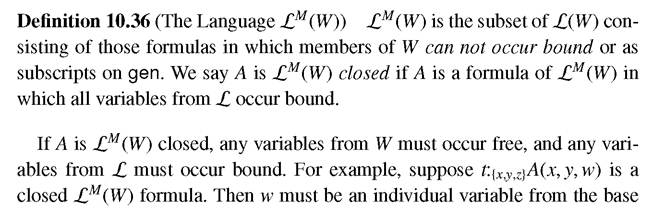
10.3.7 Completeness
We are almost ready to show that the canonical model, from Definition 10.38, does what we want. But first we sketch the details of the version of the Henkin- Lindenbaum construction that we will need. 
formulas as follows.
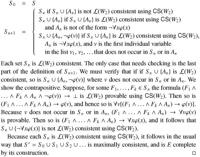
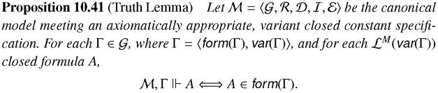
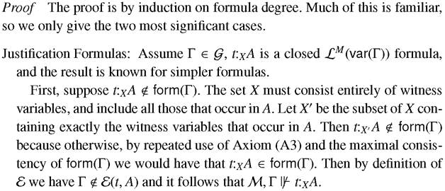
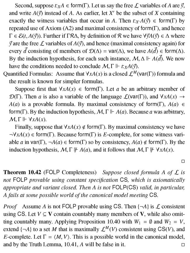
With this out of the way, a version of the familiar Truth Lemma can be shown, and then completeness is simple.
10.3.8 Fully Explanatory Models
For propositional justification logics, fully explanatory Fitting models were discussed earlier, Definition 4.4. This extends to the quantified setting very directly.
Definition 10.43 (Fully Explanatory)
is fully explanatory if it meets the following condition. Let A be an arbitrary formula with no free individual variables, but with constants from the domain of the model M, Section 10.3.2, and let Γ be an arbitrary possible world in G in which A lives. If M, A IF A for every such that ΓRΔ then
for some justification term t, where X is the set of domain constants appearing in A.
This is the direct extension of the propositional version and informally says the same thing. If A is necessary at a possible world of a fully explanatory model, in the sense that it is true at all accessible worlds, then there is a reason for it—A has a justification at that world. The following establishes that FOLP is complete with respect to the class of fully explanatory Fitting models.
Theorem 10.44 The canonical model, meeting an axiomatically appropriate, variant closed constant specification, is fully explanatory. 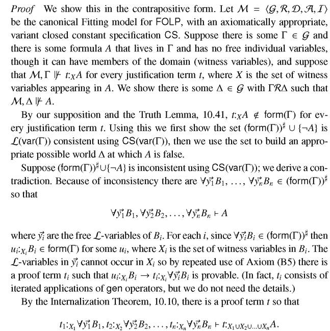
This, combined with the provability of each ui:XjBi → ti:Xi8yiBi, gives us provability of the following
Corollary 10.45 FOLP is complete with respect to the class of fully explanatory models.
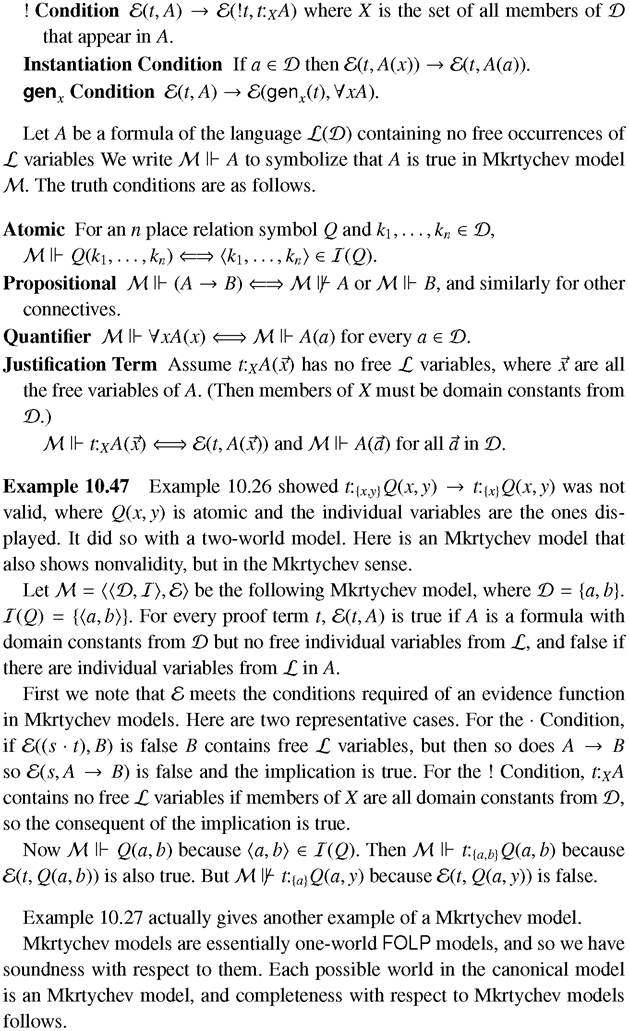
10.3.9 Mkrtychev Models
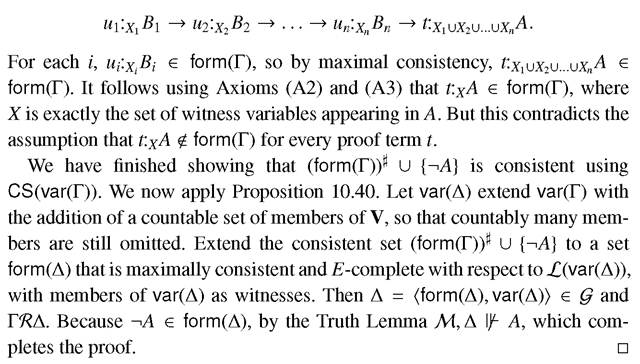
Fitting models for FOLP have both a semantic and a syntactic component. They use the semantic machinery of first-order modal models and also have an evidence function that depends on syntactic details of formulas. Possible world semantics is flexible and provides a plausible intuition, but in fact the syntactic-based approach of Mkrtychev models, Section 3.5, extends to admit quantifiers. We sketch the details.
Definition 10.46 (Mkrtychev Model) An Mkrtychev FOLP model is a struc- 
10.4