An Algebraic Version of the Classica l AD-AS Model with Misperceptions
Building on the algebraic version of the AD-AS model developed in Appendix 9.B, in this appendix we derive an algebraic version of the classical AD-AS model with misperceptions. We present algebraic versions of the aggregate demand (AD) curve and the aggregate supply (AS) curve and then solve for the general equilibrium.
The Aggregate Demand Curve
Because misperceptions by producers don't affect the demand for goods, the aggregate demand curve is the same as in Appendix 9.B. Recall from Eq. (9.B.24) that the equation of the aggregate demand (AD) curve is

where the coefficients of the IS curve, αιs and βιs, are given by Eqs. (9.B.15) and (9.B.16), respectively, the coefficients of the LM curve, αlm and eLM, are given by Eqs. (9.B.20) and (9.B.21), respectively, and L is the coefficient of the nominal interest rate in the money demand equation, Eq. (9.B.17).
The Aggregate Supply Curve
The short-run aggregate supply curve based on the misperceptions theory is represented by Eq. (10.4), which, for convenience, we repeat here:

where b is a positive number.
General Equilibrium
For a given expected price level, Pe, the short-run equilibrium value of the price level is determined by the intersection of the aggregate demand curve (Eq. 10.B.1) and the short-run aggregate supply curve (Eq. 10.B.2). Setting the right sides of Eqs. (10.B.1) and (10.B.2) equal and multiplying both sides of the resulting equation by  and rearranging yields a quadratic equation for the price level P:
where
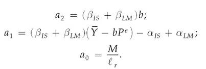
The coefficients a2 and a 0 are positive, and the coefficient a 1 could be positive, negative, or zero. Because both a 2 and a 0 are positive, the solution of Eq.
(10.B.3) yields one positive value of P and one negative value of P. The price level can't be negative, so the short-run equilibrium price level is the positive solution of this equation. Using the standard quadratic formula, we find the positive solution of Eq. (10.B.3) to be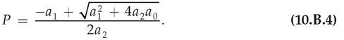
We obtain the short-run equilibrium level of output by substituting the value of the price level from Eq. (10.B.4) into either the aggregate demand curve Eq. (10.B.1) or the aggregate supply curve Eq. (10.B.2).
Note that an increase in the nominal money supply, M, increases the constant a0 and thus according to Eq. (10.B.4), it increases the equilibrium price level. Because an increase in M doesn't affect the aggregate supply curve but does increase the equilibrium price level, Eq. (10.B.2) shows that it increases output.
We focused on short-run equilibrium in this appendix. In the long run, the actual price level equals the expected price level so that, according to Eq. (10.B.2), output equals its full-employment level, Y. In the long run, the economy reaches the general equilibrium described in Appendix 9.B.