An Algebraic Version of the Open-Economy IS-LM Model

The IS-LM model for the open economy is basically the same as the closed-economy IS-LM model derived in Appendix 9.B, with the exception that the goods market equilibrium condition (the IS curve) is expanded to include net exports.

To derive the IS curve for the open economy, we begin with the equations describing desired consumption and desired investment, Eqs. (9.B.8) and (9.B.10):

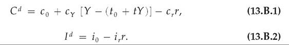
Equation (13.B.1) shows that desired consumption depends positively on dispos­able income, Y — T, and negatively on the real interest rate, r. (In Eq. 13.B.1 we used Eq. 9.B.9 to substitute for taxes, T.) Equation (13.B.2) states that desired investment depends negatively on the real interest rate, r. Other factors influenc­ing desired consumption and desired investment are included in the constant terms c ₀ and i ₀, respectively.

In an open economy net exports also are a source of demand for domestic out­put. We assume that net exports are

where x₀, x_γ, x_YF, x_r, and x_rF are positive numbers. According to Eq. (13.B.3), a country's net exports depend negatively on domestic income, Y (increased domes­tic income raises spending on imports), and positively on foreign income, Y_For (increased foreign income raises spending on exports). Net exports also depend negatively on the domestic real interest rate, r (a higher real interest rate appreci­ates the real exchange rate, making domestic goods relatively more expensive), and positively on the foreign real interest rate, r_For (a higher foreign real interest rate depreciates the domestic country's real exchange rate).

The goods market equilibrium condition for an open economy, Eq. (13.5), is

The alternative version of the open-economy goods market equilibrium condition, S^d = I^d + NX, which is emphasized in the text, could be used equally well.

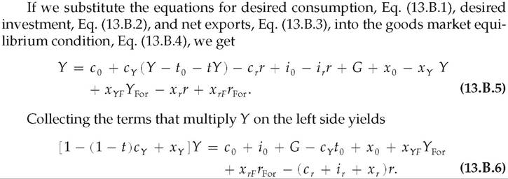
Equation (13.B.6) relates output, Y, to the real interest rate, r, that clears the goods market and thus defines the open-economy IS curve. To put Eq. (13.B.6) in a form that is easier to interpret graphically, we rewrite it with r on the left side and Y on the right side to obtain

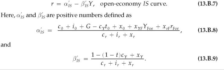
If there are no net exports, so that x ₀ = x_y = x_yf = x_r = x_rF = 0, the coefficients a_IS and PI_s reduce to the coefficients of the closed-economy IS curve, a_is and β_ιs (compare Eqs. 13.B.8 and 13.B.9 to Eqs. 9.B.15 and 9.B.16).

We use the open-economy IS curve equation, Eq. (13.B.7), to confirm the three points made about the curve in the text. pirst, it slopes downward (the slope of the IS curve is — βI_s, which is negative). Second, any factor that shifts the closed- economy IS curve also shifts the open-economy IS curve (any factor that changes the intercept a_IS also changes the intercept a^,_is in the same direction). Finally, for a given output and real interest rate, any factor that increases net exports shifts the open-economy IS curve up. That is, an increase in Y_For or r_For, or some other change that increases the demand for net exports as reflected in an increase in x ₀, raises the intercept term a_IS and thus shifts the IS curve up.

General equilibrium in the open-economy IS-LM model is determined as in the closed-economy model, except that the open-economy IS curve (Eq. 13.B.7) replaces the closed-economy IS curve (Eq. 9.B.14). Similarly, classical and Keynesian AD-AS analyses in the open economy are the same as in the closed economy (Appendix 9.B), except that the coefficients a_is and β_ιs in the equation for the aggregate demand curve, Eq. (9.B.24), are replaced by their open-economy analogues, a ^,_is and β ^,_is.

For values of output, Y, the real interest rate, r, and the price level, P, deter­mined by the open-economy IS-LM or AD-AS model, exchange rates can be determined from

where e₀, e_Y, e_YF, e_r, and e_rF are positive numbers, and

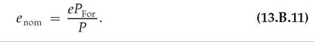
According to Eq. (13.B.10), an increase in foreign income, Y_For, or the domestic real interest rate, r—either of which raises the demand for the domestic currency in the foreign exchange market—appreciates the real exchange rate, e. Also, an increase in domestic income, Y, or the foreign real interest rate, r_For—either of which increases the supply of domestic currency in the foreign exchange market— depreciates the real exchange rate. Equation (13.B.11), which is the same as Eq. (13.6), states that the nominal exchange rate, e _nom, depends on the real exchange rate, e, and the foreign and domestic price levels, P_For and P.

To illustrate the use of Eqs. (13.B.10) and (13.B.11), let's consider the effects of a monetary expansion in the Keynesian model. In the short run an increase in the money supply raises domestic output, Y, lowers the domestic real interest rate, r, and leaves the domestic price level, P, unchanged. For these changes, Eqs. (13.B.10) and (13.B.11)—holding constant foreign output, Y_For, and the foreign real interest rate, r_For—imply a lower real exchange rate, e, and a lower nominal exchange rate, e _nom (both a real and a nominal depreciation). In the long run money is neutral, so Y and r return to their original levels. Equation (13.B.10) indicates therefore that the real exchange rate, e, also returns to its original value in the long run. However, a monetary expansion leads to a long-run increase in the domestic price level, P. Hence Eq. (13.B.11) shows that the nominal exchange rate, e _nom, also depreciates in the long run.