Appendix A A Formal Model of Consumption and Saving
This appendix analyzes more formally the decision about how much to consume and how much to save. We focus on the decisions of a consumer named Penelope. To help keep the analysis manageable, we make three simplifying assumptions:
1.
The time horizon over which Penelope makes plans consists of only two periods: the present, or current, period and the future period. The current period might represent Penelope's working years and the future period might represent her retirement years, for example.2. Penelope takes her current income, future income, and wealth as given.
3. Penelope faces a given real interest rate and can choose how much to borrow or save at that rate.
How Much Can the Consumer Afford? The Budget Constraint
To analyze Penelope's decision about how much to consume and save, we first examine the choices available to her. To have some specific numbers to analyze, let's suppose that Penelope receives a fixed after-tax income, measured in real terms,1 of 42,000 in the current period and expects to receive a real income of 33,000 in the future period. In addition, she begins the current period with real wealth of 18,000 in a savings account, and she can borrow or lend at a real interest rate of 10% per period.
Next, we list the symbols used to represent Penelope's situation:
y = Penelope's current real income (42,000);
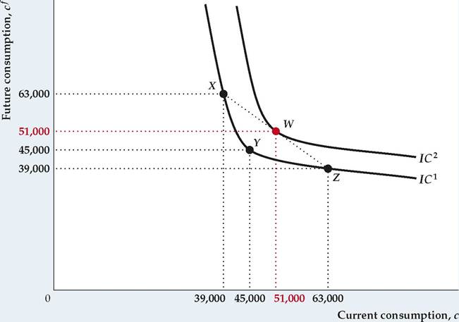
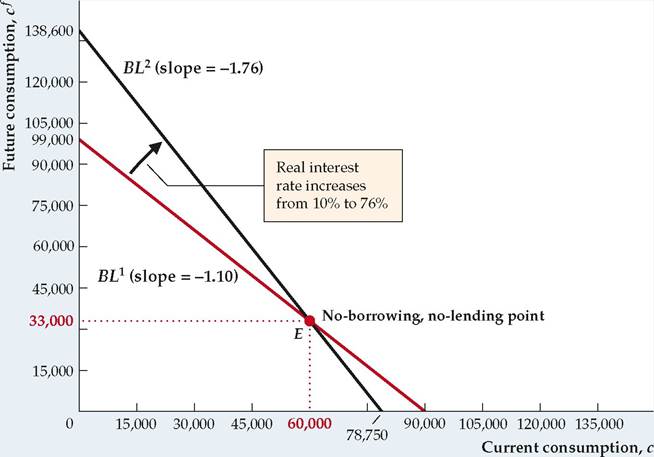
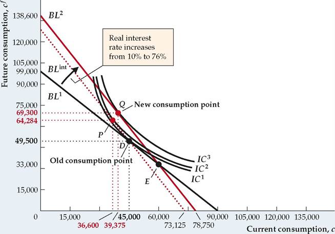
a = Penelope's real wealth (assets) at the beginning of the current period (18,000); r = real interest rate (10%); c = Penelope's current real consumption (not yet determined); cf = Penelope's future real consumption (not yet determined). In general, any amount of current consumption, c, that Penelope chooses will determine the amount of future consumption, cf, that she will be able to afford. Penelope can put these leftover current resources, y + a — c, in the bank to earn interest. If the real interest rate that she can earn on her deposit is r, the real value of her bank account (principal plus interest) in the future period will be (y + a — c)(1 + r). In addition to the real value of her bank account in the future period, Penelope receives income of yf, so her total resources in the future period Equation (4A.1) is called the budget constraint. It shows for any level of current consumption, c, how much future consumption, The budget line slopes downward, reflecting the trade-off between current and future consumption. If Penelope increases her current consumption by one unit, her saving falls by one unit. Because saving earns interest at rate r, a one-unit decline in saving today implies that Penelope's future resources—and thus her future consumption—will be lower by 1 + r units. Present Values We can conveniently represent Penelope's budget constraint by using the concept of present value. The present value measures the value of payments to be made in the future in terms of today's dollars or goods. To illustrate this concept, suppose you must make a payment of $13,200 one year from now. How much money would you have to put aside today so you could make that future payment? The answer to this question is called the present value. The present value of a future payment depends on the interest rate. If the current nominal interest rate, i, is 10% per year, the present value of $13,200 to be paid one year from now is $12,000. The reason is that $12,000 deposited in the bank today at a 10% interest rate will earn $1200 (10% of $12,000) of interest in one year, which, when added to the initial $12,000, gives the $13,200. Therefore, at an interest rate of 10%, having $13,200 one year from now is economically equivalent to having $12,000 today. Thus, we say the present value of $13,200 in one year equals $12,000. More generally, if the nominal interest rate is i per year, each dollar in the bank today is worth 1 + i dollars one year from now. To have $13,200 one year from now requires $13,200/ (1 + i) in the bank today; thus the present value of $13,200 to be paid one year from now is $13,200/ (1 + i). As we have already shown, if i = 10% per year, the present value of $13,200 one year from now is $13,200/1.10 = $12,000. If i = 20% per year, the present value of $13,200 one year in the future is $13,200/1.20 = $11,000. Hence an increase in the interest rate reduces the present value of a future payment. Similarly, a decline in the interest rate increases the present value of a future payment. If future payments are measured in nominal terms, as in the preceding example, the appropriate interest rate for calculating present values is the nominal interest rate, i. If future payments are measured in real terms, present values are calculated in exactly the same way, except that we use the real interest rate, r, rather than the nominal interest rate, i. In analyzing Penelope's consumptionsaving decision, we're measuring everything in real terms, so we use the real interest rate, r, to calculate the present values of Penelope's future income and consumption. Present Value and the Budget Constraint We define the present value of lifetime resources (PVLR) as the present value of the income that a consumer expects to receive in current and future periods plus initial wealth. In the two-period case, the present value of lifetime resources is In terms of Fig. 4.A.1, and indeed for any graph of the budget line, PVLR equals the value of current consumption, c, at the horizontal intercept of the budget line because the horizontal intercept is the point on the budget line at which future consumption, What Does the Consumer Want? Consumer Preferences FIGURE 4.A.2 Indifference curves All points on an indifference curve represent consumption combinations that yield the same level of utility. Indifference curves slope downward because a consumer can be compensated for a reduction in current consumption by an appropriate increase in future consumption. current consumption to c = 39,000. Clearly, if she reduces current consumption while maintaining future consumption at 45,000, she will suffer a reduction in utility. However, Penelope can be compensated for this reduction in current consumption by additional future consumption. Suppose that, if she increases her future consumption to cf = 63,000 when her current consumption falls to c = 39,000, so that she moves to point X, her level of utility remains unchanged. In such a case, she is indifferent between the consumption combinations at X and Y, and points X and Y must lie on the same indifference curve. In general, any change in the level of current consumption must be accompanied by a change in the opposite direction in the level of future consumption so as to keep Penelope's level of utility unchanged. Thus indifference curves, which represent consumption combinations with equal levels of utility, must slope downward from left to right. 2. Indifference curves that are farther up and to the right represent higher levels of utility. Consider for example point W, which lies above and to the right of point Y in Fig. 4.A.2. Both current consumption and future consumption are higher at W than at Y. Because Penelope obtains utility from both current and future consumption, W offers a higher level of utility than does Y; that is, Penelope prefers W to Y. 3. Indifference curves are bowed toward the origin. This characteristic shape of indifference curves captures the consumption-smoothing motive, discussed in Chapter 4. Under the consumption-smoothing motive, consumers prefer a relatively smooth pattern of consumption over time to having large amounts of consumption in one period and small amounts in another period. We can illustrate the link between the shape of indifference curves and the consumption-smoothing motive by considering the following three consumption combinations in Fig. 4.A.2: point X(c = 39,000; cf = 63,000), point W(c = 51,000; cf = 51,000) and point Z(c = 63,000; cf = 39,000). Note that W corresponds to complete consumption smoothing, with equal consumption occurring in both periods. In contrast, X and Z represent consumption combinations with large changes in consumption between the first period and the second period. In addition, note that W represents a consumption combination that is the average of the consumption combinations at X and Z: Current consumption at W, 51,000, is the average of current consumption at X and Z, 39,000 and 63,000, respectively; similarly, future consumption at W, also 51,000, is the average of future consumption at X and Z, 63,000 and 39,000, respectively. Even though point W essentially is an average of points X and Z, and Penelope is indifferent between X and Z, she prefers W to X and Z because W represents much "smoother" (more even) consumption. Graphically, her preference for W over X and Z is indicated by W's position above and to the right of indifference curve IC[73] (which runs through X and Z). Note that W lies on a straight line drawn between X and Z. The only way that W can lie above and to the right of IC1 is if IC1 bows toward the origin, as depicted in Fig. 4.A.2. Thus the bowed shape of the indifference curve reflects the consumption-smoothing motive. The Optimal Level of Consumption FIGURE 4.A.3 The optimal consumption combination The optimal (highest utility) combination of current and future consumption is represented by the point of tangency between the budget line and an indifference curve (point D). All other points on the budget line, such as B and E, lie on indifference curves below and to the left of indifference curve IC* and thus yield lower utility than the consumption combination at D, which lies on IC*. Penelope would prefer the consumption combination at point T to the one at D, but as T lies above the budget line she can't afford the consumption combination that T represents. The Effects of Changes in Income and Wealth on Consumption and Saving The formal model developed in this appendix provides a helpful insight: The effect on consumption of a change in current income, expected future income, or wealth depends only on how that change affects the consumer's present value of lifetime resources, PVLR. An Increase in Current Income Suppose that Penelope receives a bonus at work of 12,000, which raises her current real income from 42,000 to 54,000. Her initial assets (18,000), future income (33,000), and the real interest rate (10%) remain unchanged; hence the increase of 12,000 in current income implies an equal increase in Penelope's present value of lifetime resources, or PVLR. If she hasn't yet committed herself to her original consumption-saving plan, how might Penelope revise that plan in light of her increased current income? We use the graph in Figure 4.A.4 to answer this question. In Fig. 4.A.4, BL1 is Penelope's original budget line, and point D, where c = 45,000 and cf = 49,500 represents Penelope's original, pre-bonus consumption plan. Penelope's bonus will allow her to consume more, both now and in the future, so the increase in her income causes her budget line to shift. To see exactly how it shifts, note that the increase of 12,000 in Penelope's current income implies that her PVLR also increases by 12,000. Because the horizontal intercept of the budget line occurs at c = PVLR, the bonus shifts the horizontal intercept to the right by 12,000. The slope of the budget line, — (1 + r) = —1.10, remains unchanged because the real interest rate r is unchanged. Thus the increase in current income of 12,000 causes a parallel shift of the budget line to the right by 12,000, from BL1 to BL2. FIGURE 4.A.4 An increase in income or wealth An increase in current income, future income, and/or initial wealth that raises Penelope's PVLR by 12,000 causes the budget line to make a parallel shift to the right by 12,000, from BL1 to BL2. If Penelope's original consumption plan was to consume at point D, she could move to point H by spending all the increase on future consumption and none on current consumption; or she could move to point K by spending all the increase on current consumption and none on future consumption. However, if Penelope has a consumption-smoothing motive she will move to point J, which has both higher current consumption and higher future consumption than D. Point J is optimal because it lies where the new budget line BL2 is tangent to an indifference curve, IC**. That shift demonstrates graphically that, after receiving her bonus, Penelope can enjoy greater current and future consumption. One strategy for Penelope, represented by point K on the new budget line BL2, is to use the entire bonus to increase her current consumption by 12,000 while leaving her future consumption unchanged. Another strategy, represented by point H on BL2, is to save all of her bonus while keeping her current consumption unchanged, and then use both the bonus and the interest of 1,200 earned on the bonus to increase her future consumption by 13,200. If Penelope operates under a consumption-smoothing motive, she will use her bonus to increase both her current consumption and (by saving part of her bonus) her future consumption, thereby choosing a point on BL2 between point K (consume the entire bonus) and point H (save the entire bonus). If her indifference curves are as shown in Fig. 4.A.4, she will move to J, where her new budget line, BL2, is tangent to the indifference curve IC**. At J, current consumption, c, is 51,000, future consumption, cf, is 56,100, and saving, s, is 54,000 — 51,000 = 3000. Both current and future consumption are higher at J than at D (where c = 45,000 and cf = 49,500). Penelope's current saving of 3000 at J is higher than her saving was at D (where she dissaved by 3000) because the increase in her current consumption of 6000 is less than the increase in her current income of 12,000. This example illustrates that an increase in current income raises both current consumption and current saving. An Increase in Future Income Suppose that Penelope doesn't receive her bonus of 12,000 in the current period, so that her current income, y, remains at its initial level of 42,000. Instead, because of an improved company pension plan, she learns that her future income will increase by 13,200, so yf rises from 33,000 to 46,200. How will this good news affect Penelope's current consumption and saving? At a real interest rate of 10%, the improvement in the pension plan increases the present value of Penelope's future income by 13,200/1.10, or 12,000. So, as in the case of the current-period bonus just discussed, the improved pension plan raises Penelope's PVLR by 12,000 and causes a parallel shift of the budget line to the right by that amount. The effects on current and future consumption are therefore exactly the same as they were for the increase of 12,000 in current income (and Fig. 4.A.4 applies equally well here). Although increases in current income and expected future income that are equal in present value will have the same effects on current and planned future consumption, the effects of these changes on current saving are different. Previously, we showed that an increase in current income raises current saving. In contrast, because the increase in future income raises current consumption (by 6000 in this example) but doesn't affect current income, it causes saving to fall (by 6000, from -3000 to -9000). Penelope knows that she will be receiving more income in the future, so she has less need to save today. An Increase in Wealth Changes in wealth also affect consumption and saving. As in the cases of current and future income, the effect of a change in wealth on consumption depends only on how much the PVLR changes. For example, if Penelope finds a passbook savings account in her attic worth 12,000, her PVLR increases by 12,000. To illustrate this situation, we use Fig. 4.A.4 again. Penelope's increase in wealth raises her PVLR by 12,000 and thus shifts the budget line to the right by 12,000, from BL1 to BL2. As before, her optimal consumption choice goes from point D (before she finds the passbook) to point J (after her increase in wealth). Because the increase in wealth raises current consumption (from 45,000 at D to 51,000 at J) but leaves current income (42,000) unchanged, it results in a decline in current saving (from -3000 at D to -9000 at J). Being wealthier, Penelope does not have to save as much of her current income (actually, she is increasing her dissaving) to provide for the future. The preceding analyses show that changes in current income, future income, and initial wealth all lead to parallel shifts of the budget line by the amount that they change the PVLR. Economists use the term income effect to describe the impact of any change that causes a parallel shift of the budget line. The Permanent Income Theory In terms of our model, a temporary increase in income represents a rise in current income, y, with future income, y f, held constant. A permanent increase in income raises both current income, y, and future income, yf. Therefore a permanent one- unit increase in income leads to a larger increase in PVLR than does a temporary one-unit increase in income. Because income changes affect consumption only to the extent that they lead to changes in PVLR, our theory predicts that a permanent one-unit increase in income will raise current and future consumption more than a temporary one-unit increase in income will. This distinction between the effects of permanent and temporary income changes is emphasized in the permanent income theory of consumption and saving, developed in the 1950s by Nobel laureate Milton Friedman. He pointed out that income should affect consumption only through the PVLR in a many-period version of the model we present here. Thus permanent changes in income, because they last for many periods, may have much larger effects on consumption than temporary changes in income. As a result, temporary income increases would be mostly saved, and permanent income increases would be mostly consumed.[74] Consumption and Saving over Many Periods: The Life-Cycle Model The two-period model suggests that a significant part of saving is intended to pay for retirement. However, it doesn't reflect other important aspects of a consumer's lifetime income and consumption patterns. For example, income typically rises over most of a person's working life, and people save for reasons other than retirement. The life-cycle model of consumption and saving, originated in the 1950s by Nobel laureate Franco Modigliani and his associates, extends the model from two periods to many periods and focuses on the patterns of income, consumption, and saving throughout an individual's life. The essence of the life-cycle model is shown in Figure 4.A.5. In Fig. 4.A.5(a), the typical consumer's patterns of income and consumption are plotted against the consumer's age, from age 20 (the approximate age of economic independence) to age 90 (the approximate age of death). Two aspects of Fig. 4.A.5(a) are significant. First, the average worker experiences steadily rising real income, with peak earnings typically occurring between the ages of 50 and 60. After retirement, income (excluding interest earned from previous saving) drops sharply. Second, the lifetime pattern of consumption is much smoother than the pattern of income over time, which is consistent with the consumption-smoothing motive discussed earlier. Although shown as perfectly flat in Fig. 4.A.5(a), consumption, in reality, varies somewhat by age; for example, it will be higher during years of high child-rearing expenses. An advantage of using the life-cycle model to study consumption and saving is that it may be easily modified to allow for various patterns of lifetime income and consumption. The lifetime pattern of saving, shown in Fig. 4.A.5(b), is the difference between the income and consumption curves in Fig. 4.A.5(a). This overall hump-shaped pattern has been confirmed empirically. Saving is minimal or even negative during the early working years, when income is low. Maximum saving occurs when the worker is between ages 50 and 60, when income is highest. Finally, dissaving occurs during retirement as the consumer draws down accumulated wealth to meet living expenses. An important implication of the hump-shaped pattern of saving is that national saving rates depend on the age distribution of a country's population. Countries with unusually young or unusually old populations have low saving rates, and countries with relatively more people in their middle years have higher saving rates. Bequests and Saving We have assumed that the consumer plans to spend all of his or her wealth and income during his or her lifetime, leaving nothing to heirs. In reality, many people leave bequests, or inheritances, to children, charities, and others. To the extent that FIGURE 4.A.5 Life-cycle consumption, income, and saving (a) Income and consumption are plotted against age. Income typically rises gradually throughout most of a person's working life and peaks shortly before retirement. The desire for a smooth pattern of consumption means that consumption varies less than income over the life cycle. Consumption here is constant. (b) Saving is the difference between income and consumption; the saving pattern is hump-shaped. Early in a person's working life consumption is larger than income, so saving is negative. In the middle years saving is positive; the excess of income over consumption is used to repay debts incurred earlier in life and to provide for retirement. During retirement people dissave. revenue has been reduced by 300 and its expenditures have not changed, however, the government must increase its current borrowing from the public by 300 (per taxpayer). Furthermore, the government must pay interest on its borrowings. For example, if the real interest rate that the government must pay on its debt is 10%, in the future period the government's outstanding debt will be 330 greater than it would have been without the tax cut. consumers desire to leave bequests, they will consume less and save more than when they simply consume all their resources during their lifetimes. Ricardian Equivalence One of the most significant results of analyzing our model is that changes in income or wealth affect desired consumption only to the extent that they affect the consumer's PVLR. The point made by advocates of Ricardian equivalence, discussed in Chapter 4, is that, holding current and future government purchases constant, a change in current taxes does not affect the consumer's PVLR and thus should not affect desired consumption, Cd, or desired national saving, Y — Cd — G. To illustrate this idea, suppose that the government cuts Penelope's current taxes by 300. This tax reduction increases Penelope's current income by 300, which (all else being equal) would cause her to consume more. Because the government's As a taxpayer, Penelope is ultimately responsible for the government's debts. Suppose that the government decides to repay its borrowings and accumulated interest in the future period. (Chapter 15 discusses what happens if the government's debt is left for Penelope's descendants to repay.) To repay its debt plus interest, the government must raise taxes in the future period by 330, so Penelope's expected future income falls by 330. Overall, then, the government's tax program has raised Penelope's current income by 300 but reduced her future income by 330. At a real interest rate of 10%, the present value of the future income change is -300, which cancels out the increase in current income of 300. Thus Penelope's PVLR is unchanged by the tax cut, and (as the Ricardian equivalence proposition implies) she should not change her current consumption. Excess Sensitivity and Borrowing Constraints A variety of studies have confirmed that consumption is affected by current income, expected future income, and wealth, and that permanent income changes have larger effects on consumption than temporary income changes— all of which are outcomes implied by the model. Nevertheless, some studies show that the response of consumption to a change in current income is greater than would be expected on the basis of the effect of the current income change on PVLR. This tendency of consumption to respond to current income more strongly than the model predicts is called the excess sensitivity of consumption to current income. One explanation for excess sensitivity is that people are more short-sighted than assumed in our model and thus consume a larger portion of an increase in current income than predicted by it. Another explanation, which is more in the spirit of the model, is that the amount that people can borrow is limited. A restriction imposed by lenders on the amount that someone can borrow against future income is called a borrowing constraint. The effect of a borrowing constraint on the consumption-saving decision depends on whether the consumer would want to borrow in the absence of a borrowing constraint. If the consumer wouldn't want to borrow even if borrowing were possible, the borrowing constraint is said to be nonbinding. When a consumer wants to borrow but is prevented from doing so, the borrowing constraint is said to be binding. A consumer who faces a binding borrowing constraint will spend all available current income and wealth on current consumption so as to come as close as possible to the consumption combination desired in the absence of borrowing constraints. Such a consumer would consume the entire amount of an increase in current income. Thus the effect of an increase in current income on current consumption is greater for a consumer who faces a binding borrowing constraint than is predicted by our simple model without borrowing constraints. In macroeconomic terms, this result implies that—if a significant number of consumers face binding borrowing constraints—the response of aggregate consumption to an increase in aggregate income will be greater than implied by the basic theory in the absence of borrowing constraints. In other words, if borrowing constraints exist, consumption may be excessively sensitive to current income.[75] The Real Interest Rate and the Consumption-Saving Decision To explore the effects of a change in the real interest rate on consumption and saving, let's return to the two-period model and Penelope's situation. Recall that Penelope initially has current real income, y, of 42,000, future income, yf, of 33,000, initial wealth, a, of 18,000, and that she faces a real interest rate, r, of 10%. Her budget line, which is the same as in Fig. 4.A.1, is shown in Figure 4.A.6 as BL1. Now let's see what happens when for some reason the real interest rate jumps from 10% to 760%.[76] FIGURE 4.A.6 The effect of an increase in the real interest rate on the budget line The figure shows the effect on Penelope's budget line of an increase in the real interest rate, r, from 10% to 76%. Because the slope of a budget line is —(1 + r) and the initial real interest rate is 10%, the slope of Penelope's initial budget line, BL1, is -1.10. The initial budget line, BL1, also passes through the no-borrowing, no-lending point, E, which represents the consumption combination that Penelope obtains by spending all her current income and wealth on current consumption. Because E can still be obtained when the real interest rate rises, it also lies on the new budget line, BL2. However, the slope of BL2 is -1.76, reflecting the rise in the real interest rate to 76%. Thus the higher real interest rate causes the budget line to pivot clockwise around the no-borrowing, no-lending point. The Real Interest Rate and the Budget Line To see how Penelope's budget line is affected when the real interest rate rises, let's first consider point E on the budget line BL1. Point E is special in that it is the only point on the budget line at which current consumption equals current income plus initial wealth (c = y + a = 60,000) and future consumption equals future income (cf = yf = 33,000). If Penelope chooses this consumption combination, she doesn't need to borrow (her current income and initial wealth are just sufficient to pay for her current consumption), nor does she have any current resources left to deposit in (lend to) the bank. Thus E is the no-borrowing, no-lending point. Because E involves neither borrowing nor lending, the consumption combination it represents is available to Penelope regardless of the real interest rate. Thus the no-borrowing, no-lending point remains on the budget line when the real interest rate changes. Next, recall that the budget line's slope is —(1 + r). When the real interest rate, r, jumps from 10% to 76%, the slope of the budget line changes from -1.10 to -1.76; that is, the new budget line becomes steeper. Because the budget line becomes steeper but still passes through the no-borrowing, no-lending point, E, it pivots clockwise around point E. The Substitution Effect As we discussed in Chapter 4, the price of current consumption in terms of future consumption is 1 + r because if Penelope increases her consumption by one unit today, thereby reducing her saving by one unit, she will have to reduce her future consumption by 1 + r units. When the real interest rate increases, current consumption becomes more expensive relative to future consumption. In response to this increase in the relative price of current consumption, Penelope substitutes away from current consumption toward future consumption by increasing her saving. This increase in saving reflects the substitution effect of the real interest rate on saving, introduced in Chapter 4. The substitution effect is illustrated graphically in Figure 4.A.7. Initially, the real interest rate is 10% and the budget line is BL1. Suppose for now that Penelope's preferences are such that BL1 is tangent to an indifference curve, IC1, at the no-borrowing, no-lending point, E.[77] At a real interest rate of 10%, Penelope chooses the consumption combination at E. When the real interest rate rises from 10% to 76%, the budget line pivots clockwise to BL2. Because Penelope's original consumption point—the no-borrowing, no-lending point, E—also lies on the new budget line, BL2, she has the option of remaining at E and enjoying the same combination of current and future consumption after the real interest rate rises. Points along BL2 immediately above and to the left of E lie above and to the right of IC1, however. These points represent consumption combinations that are available to Penelope and yield a higher level of utility than the consumption combination at E. Penelope can attain the highest level of utility along BL2 at point V, where indifference curve IC2 is tangent to BL2. In response to the increase in the relative price of current consumption, Penelope reduces her current consumption, from 60,000 to 51,000, and moves from E to V on BL2. Her reduction of 9000 in current consumption between E and V is equivalent to an increase of 9000 in saving. The increase in saving between E and V reflects the substitution effect on saving of a higher real interest rate. The Income Effect If Penelope's current consumption initially equals her current resources (current income plus initial wealth) so that she is neither a lender nor a borrower, a change in the real interest rate has only a substitution effect on her saving, as shown in Fig. 4.A.7. If her current consumption initially is not equal to her current resources, FIGURE 4.A.7 The substitution effect of an increase in the real interest rate We assume that Penelope's preferences are such that when the real interest rate is 10%, she chooses the consumption combination at the no-borrowing, no-lending point, E, on the initial budget line BL1. Point E lies on the indifference curve IC1. An increase in the real interest rate to 76% causes the budget line to pivot clockwise from BL1 to BL2, as in Fig. 4.A.6. By substituting future consumption for current consumption along the new budget line, BL2, Penelope can reach points that lie above and to the right of IC1; these points represent consumption combinations that yield higher utility than the consumption combination at E. Her highest utility is achieved by moving to point V, where the new budget line, BL2, is tangent to indifference curve IC2. The drop in current consumption (by 9000) and the resulting equal rise in saving that occur in moving from E to V reflect the substitution effect of the increase in the real interest rate. however, then an increase in the real interest rate also has an income effect. As we discussed in Chapter 4, if Penelope is initially a saver (equivalently, a lender), with current consumption less than her current resources (current income plus initial wealth), an increase in the real interest rate makes her financially better off by increasing the future interest payments that she will receive. In response to this increase in future interest income, she increases her current consumption and reduces her current saving. On the other hand, if Penelope is initially a borrower, with current consumption exceeding her current resources, an increase in the real interest rate increases the interest she will have to pay in the future. Having to make higher interest payments in the future makes Penelope financially worse off overall, leading her to reduce her current consumption. Thus, for a borrower, the income effect of an increase in the real interest rate leads to reduced current consumption and increased saving. The Substitution Effect and the Income Effect Together Figure 4.A.8 illustrates the full impact of an increase in the real interest rate on Penelope's saving, including the substitution and income effects—assuming that Penelope initially is a lender. As before, Penelope's original budget line is BL1 when the real interest rate is 10%. We now assume that Penelope's preferences are such that BL1 is tangent to an indifference curve, IC1, at point D. Thus, at a 10% real interest rate, Penelope plans current consumption of 45,000 and future consumption of 49,500. Her current resources equal 60,000 (current income of 42,000 plus initial assets of 18,000), so if she enjoys current consumption of 45,000 she will have resources of 15,000 to lend. Her chosen point, D, is located to the left of the no-borrowing, no-lending point, E (current consumption is lower at D than at E), showing that Penelope is a lender. The increase in the real interest rate from 10% to 76% causes Penelope's budget line to pivot clockwise through the no-borrowing, no-lending point, E, ending FIGURE 4.A.8 An increase in the real interest rate with both an income effect and a substitution effect We assume that Penelope initially consumes at point D on the original budget line, BL1. An increase in the real interest rate from 10% to 76% causes the budget line to pivot clockwise, from BL1 to the new budget line, BL2. We break the overall shift of the budget line into two parts: (1) a pivot around the original consumption point, D, to yield an intermediate budget line, BLint, and (2) a parallel shift from BLint to the final budget line, BL2. The substitution effect is measured by the movement from the original consumption point, D, to point P on BLint, and the income effect is measured by the movement from P to Q on BL2. As drawn, the substitution effect is larger than the income effect so that the overall effect is for current consumption to fall and saving to rise. at BL2 as before. To separate the substitution and income effects of the increase in the real interest rate, think of the movement of the budget line from BL1 to BL2 as taking place in two steps. First, imagine that the original budget line, BL1, pivots clockwise around Penelope's original consumption combination, point D, until it is parallel to the new budget line, BL2 (that is, its slope is -1.76). The resulting intermediate budget line is the dotted line, BLint. Second, imagine that BLint makes a parallel shift to the right to BL2. The response of Penelope's saving and current consumption to the increase in the real interest rate can also be broken into two steps. First, consider her response to the pivot of the budget line through point D, from BL1 to BLint. If this change were the only one in Penelope's budget line, she would move from D to P (c = 36,600 and cf = 64,284) on BLint. At P, she would save more and enjoy less current consumption than at D. The increase in saving between D and P, similar to Penelope's shift from E to V in Fig. 4.A.7, measures the substitution effect on Penelope's saving of the increase in the real interest rate. Second, consider the effect of the parallel shift from BLint to BL2. The new budget line, BL2, is tangent to an indifference curve, IC3, at point Q, so Penelope will choose the consumption combination at Q. Current and future consumption are higher, and saving is lower, at Q than at P. The increase in current consumption and the decrease in saving between P and Q reflect the income effect of the increase in the real interest rate. Thus, as discussed earlier, income effects occur when a change in some variable causes a parallel shift of the budget line. The total change in Penelope's consumption and saving resulting from the rise in the real interest rate is depicted in Fig. 4.A.8 as the change in saving between point D and point Q. This change is the sum of the substitution effect, measured by the increase in saving in moving from D to P, and the income effect, measured by the decline in saving in moving from P to Q. In Fig. 4.A.8, current consumption is lower and saving is higher at the final point, Q, than at the original point, D. However, we could just as easily draw the curves so that saving is less at the final point, Q, than at the initial point, D. Thus the theory fails to predict whether Penelope's saving will rise or fall in response to an increase in the real interest rate because the income and substitution effects work in opposite directions for a lender. As we discussed in Chapter 4, for a borrower the income and substitution effects work in the same direction. (Analytical Problem 6 at the end of Chapter 4 asks you to explain this result.) A higher real interest rate increases a borrower's reward for saving (equivalently, it increases the relative price of current consumption), so he or she tends to save more (the substitution effect); because a borrower pays rather than receives interest, a higher real interest rate also makes him or her poorer, leading to less consumption and more saving. To summarize, the two-period model implies that an increase in the real interest rate increases saving by borrowers. Nevertheless, because of conflicting income and substitution effects, economic theory isn't decisive about the effect of the real interest rate on the saving of lenders. As we discussed in Chapter 4, empirical studies have shown that an increase in the real interest rate tends to increase desired national saving, though this effect is not strong.
 = Penelope's future real income (33,000)[71] [72];
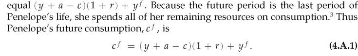
 , Penelope can afford based on her current and future income and initial wealth.4 The budget constraint in Eq (4.A.1) is represented graphically by the budget line, which shows the combinations of current and future consumption that Penelope can afford, based on her current and future income, her initial level of wealth, and the real interest rate. Figure 4.A.1 depicts Penelope's budget line, with current consumption, c, on the horizontal axis and future consumption, cf, on the vertical axis.
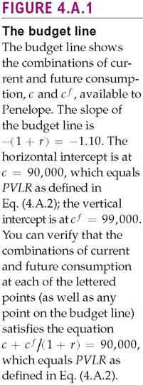

 , equals zero. Setting future consumption,
 to zero in Eq. (4.A.3) yields current consumption, c, on the left side of the equation, which must equal PVLR on the right side. Thus c = PVLR at the horizontal intercept of the budget line.