Appendix A Some Useful Analytical Tools
In this appendix we review some basic algebraic and graphical tools used in this book.
A.1 Functions and Graphs
A function is a relationship among two or more variables.
For an economic illustration of a function, suppose that in a certain firm each worker employed can produce five units of output per day. LetN = the number of workers employed by the firm;
Y = total daily output of the firm.
In this example, the relationship of output, Y, to the number of workers, N, is
Y = 5N. (A.1)
Equation (A.1) is an example of a function relating the variable Y to the variable N. Using this function, for any number of workers, N, we can calculate the total amount of output, Y, that the firm can produce each day. For example, if N = 3, then Y = 15.
Functions can be described graphically as well as algebraically. The graph of the function Y = 5N, for values of N between 0 and 16, is shown in Fig. A.1. Output, Y, is shown on the vertical axis, and the number of workers, N, is shown on the horizontal axis. Points on the line 0AB satisfy Eq. (A.1). For example, at point A, N = 4and Y = 20, a combination of N and Y that satisfies Eq. (A.1). Similarly, at point B, N = 12.5 and Y = 62.5, which also satisfies the relationship Y = 5N. Note that (at B, for example) the relationship between Y and N allows the variables to have values that are not whole numbers. Allowing fractional values of N and Y is reasonable because workers can work part-time or overtime, and a unit of output may be only partially completed during a day.
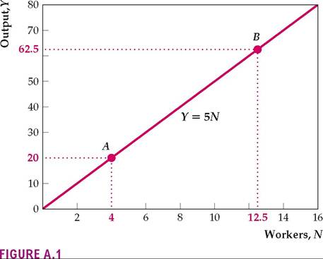
Points on the line 0AB satisfy the relationship Y = 5N. Because the graph of the function Y = 5N is a straight line, this function is called a linear function.
Equation (A.3) states that there is some general relationship between the number of workers, N, and the amount of output, Y, which is represented by a function, G.
The numerical functions given in Eqs. (A.1) and (A.2) are specific examples of such a general relationship.
A.2 Slopes of Functions
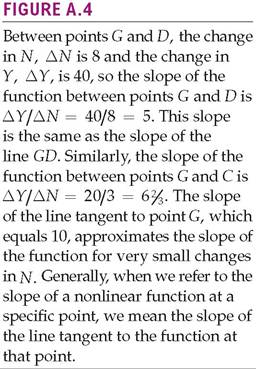
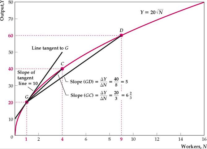
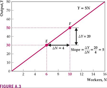
of the increase in ∆N being considered. The slope of a nonlinear function also depends on the point at which the slope is being measured. In Fig. A.4 note that the slope of a line drawn tangent to point D, for example, would be less than the slope of a line drawn tangent to point G. Thus the slope of this particular function (measured with respect to small changes in N) is greater at G than at D.
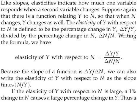
A.3 Elasticities
[1]Showing that the slope of the line tangent to point G equals 10 requires basic calculus. The derivative of the function Y = 2(F∕N, which is the same as the slope, is dY∣dN = 10^J~N. Evaluating this derivative at N = 1 yields a slope of 10.
large elasticity of Y with respect to N means that Y is very sensitive to changes in N.
A.4 Functions of Several Variables
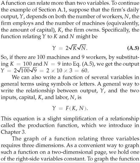
in Eq. (A.5), for example, we might hold the number of machines, K, constant at a value of 100. If we substitute 100 for K, Eq. (A.5) becomes

With K held constant at 100, Eq.
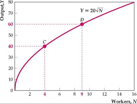
(A.6) is identical to Eq. (A.2). Like Eq. (A.2), Eq. (A.6) is a relationship between Y and N only and thus can be graphed in two dimensions. The graph of Eq. (A.6), shown as the solid curve in Fig. A.5, is identical to the graph of Eq. (A.2) in Fig. A.2.A.5 Shifts of a Curve
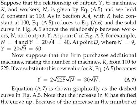
FIGURE A.5___________________________
Suppose that output, Y, depends on capital, K, and workers, N, according to the function in Eq. (A.5). If we hold K fixed at 100, the relationship between Y and N is shown by the solid curve. If K rises to 225, so that more output can be produced with a given number of workers, the curve showing the relationship between Y and N shifts up, from the solid curve to the dashed curve. In general, a change in any right-side variable that doesn't appear on an axis of the graph causes the curve to shift.
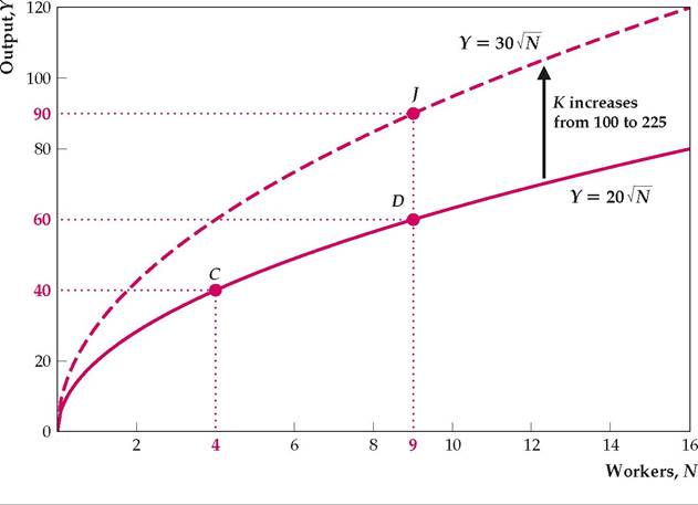
machines, the amount of daily output, Y, that can be produced for any given number of workers, N, has risen. For example, initially when N equaled 9, output, Y, equaled 60 (point D in Fig. A.5).After the increase in K, if N = 9, then
This example illustrates some important general points about the graphs of functions of several variables.
1. To graph a function of several variables in two dimensions, we hold all but one of the right-side variables constant.
2. The one right-side variable that isn't held constant (N in this example) appears on the horizontal axis. Changes in this variable don't shift the graph of the function. Instead, changes in the variable on the horizontal axis represent movements along the curve that represents the function.
3. The right-side variables held constant for the purpose of drawing the graph (K in this example) don't appear on either axis of the graph.
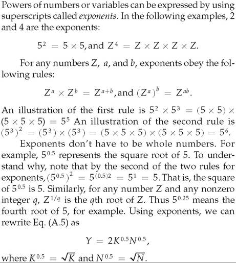
If the value of one of these variables is changed, the entire curve shifts. In this example, for any number of workers, N, the increase in machines, K, means that more output, Y, can be produced. Thus the curve shifts up, from the solid curve to the dashed curve in Fig. A.5.A.6 Exponents
A.7 Growth Rate Formulas
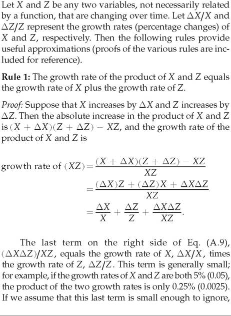
(A.9)

The real value of any asset—say, a savings account— equals the nominal or dollar value of the asset divided by the price level:
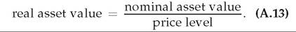
The real value of an asset is the ratio of the nominal asset value to the price level, so, according to Rule 2, the growth rate of the real asset value is approximately equal to the growth rate of the nominal asset value minus the growth rate of the price level. The growth rate of the real value of an interest-bearing asset equals the real interest rate earned by that asset; the growth rate of the nominal value of an interest-bearing asset is the nominal interest rate for that asset; and the growth rate of the price level is the inflation rate. Therefore Rule 2 implies the relationship
real interest rate = nominal interest rate — inflation rate, which is the relationship given in Eq. (2.13).
Problems
a. Suppose that N = 100. Give the function that relates Y to K and graph this relationship for 0 ≤ K ≤ 50. (You need calculate only enough values of Y to get a rough idea of the shape of the function.)
b. What happens to the function relating Y and K and to the graph of the relationship if N rises to 200? If N falls to 50? Give an economic interpretation.
c. For the function relating Y to K and N, find the elasticity of Y with respect to K and the elasticity of Y with respect to N.
5. Use a calculator to find each of the following:
6. a. Nominal GDP equals real GDP times the GDP
deflator (see Section 2.4). Suppose that nominal GDP growth is 12% and real GDP growth is 4%. What is inflation (the rate of growth of the GDP deflator)?
b. The “velocity of money," V, is defined by the equationid="Picutre 487" class="lazyload" data-src="/files/uch_group77/uch_pgroup317/uch_uch7363/image/image486.jpg">
where P is the price level, Y is real output, and M is the money supply (see Eq. 7.4). In a particular year velocity is constant, money growth is 10%, and inflation (the rate of growth of the price level) is 7%. What is real output growth?
c. Output, Y, is related to capital, K, and the number of workers, N, by the function
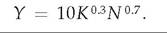
In a particular year the capital stock grows by 2% and the number of workers grows by 1%. By how much does output grow?