Comparative Dynamics
In this section, we briefly undertake some simple “comparative dynamic” exercises. By comparative dynamics, we refer to the analysis of the dynamic response of an economy to a change in its parameters or to shocks.
Comparative dynamics are different from comparative statics in Propositions 2.3, 2.8 or 2.12 in that we are interested in the entire path of adjustment of the economy following the shock or changing parameter. The basic Solow model is particularly well suited to such an analysis because of its simplicity. Such an exercise is also useful because the basic Solow model, and its neoclassical cousin, are often used for analysis of policy changes, medium-run shocks and business cycle dynamics, so understanding of how the basic model response to various shocks is useful for a range of applications. We will see in Chapter 8 that comparative dynamics are more interesting in the neoclassical growth model than the basic Solow model. Consequently, the analysis here will be brief and limited to a diagrammatic exposition. Moreover, for brevity we will focus on the continuous time economy.Recall that the law of motion of the effective capital-labor ratio in the continuous time Solow model is given by (2.46) k (t) /k (t) = sf (k (t)) /k (t) — (δ + g + n). The right-hand side of this equation is plotted in Figure 2.13. The intersection with the horizontal axis gives the steady state (balanced growth) equilibrium, k*. This figure is sufficient for us to carry out comparative dynamic exercises. Consider, for example, a one-time, unanticipated, permanent increase in the saving rate from s to s'. This shifts to curve to the right as shown by the dotted line, with a new intersection with the horizontal axis, k**. The arrows on the horizontal axis show how the effective capital-labor ratio adjusts gradually to the new balanced growth effective capital-labor ratio, k**.
Immediately, when the increase in the 76saving rate is realized, the capital stock remains unchanged (since it is a state variable). After this point, it follows the dashed arrows on the horizontal axis.
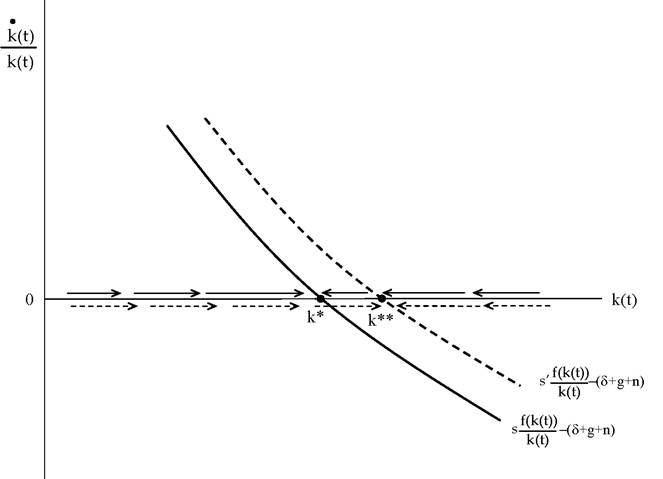
Figure 2.13. Dynamics following an increase in the savings rate from s to s'. The solid arrows show the dynamics for the initial steady state, while the dashed arrows show the dynamics for the new steady state.
The comparative dynamics following a one-time, unanticipated, permanent decrease in δ or n are identical.
We can also use the diagrammatic analysis to look at the effect of an unanticipated, but transitory change in parameters. For example, imagine that s changes in unanticipated manner at t = t', but this change will be reversed and the saving rate will return back to its original value at some known future date t = t" > t'. In this case, starting at t', the economy follows the rightwards arrows until t'. After t'', the original steady state of the differential equation applies and together with this the leftwards arrows become effective. Thus from t" onwards, the economy gradually returns back to its original balanced growth equilibrium, k*.
We will see that similar comparative dynamics can be carried out in the neoclassical growth model as well, but the response of the economy to some of these changes will be more complex.
2.7.