Dynamic Programming with Expectations
We use a notation similar to that in Chapter 6. Let us first introduce the stochastic (random) variable z (t) ∈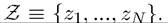 _ Note that the set Z is finite and thus compact,
which will simplify the analysis considerably.
Let the instantaneous payoff at time t be U(x (t),x (t + 1),z (t)), where x (t) ∈ X ⊂ Rk for some K ≥ 1 and U : X ? X ? Z → R. This extends the payoff function in Chapter 6, which took the form U(x (t),x (t + 1)), by making payoffs directly a function of the stochastic variable z (t). As usual, returns will be discounted by some discount factor β ∈ (0,1). The initial value x (0) is given. We will again think of x (t) as the state variable (state vector) and of x (t + 1) as the control variable (control vector) at time t.An additional difference from Problem A1 in Chapter 6 is that the constraint on x (t + 1) is no longer of the form x (t + 1) ∈ G(x (t)). Instead, the constraint also incorporates the stochastic variable z (t) and is written as
x (t + 1) ∈ G (x (t),z (t)),
where again G(x, z) is a set-valued mapping or a correspondence 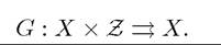
We assume that the stochastic variable z (t) follows a (first-order) Markov chain.[33] The important property implied by the Markov chain assumption is that the current value of z (t) only depends on its last period value, z (t — 1). Mathematically, this can be expressed as

The simplest example of an economic model with uncertainty represented by a Markov chain would be one in which the stochastic variable takes finitely many values and is independently distributed over time.
In this case, clearly,
and the Markov property is trivially satisfied. More generally, however, Markov chains enable us to model economic environments in which stochastic shocks are correlated over time. Markov chains are widely used in the theory of probability, in research in stochastic processes and in various areas of dynamic economic analysis. While the theory of Markov chains is relatively straightforward, not much of this theory is necessary for the basic treatment of stochastic dynamic programming here.
The Markov property not only simplifies the mathematical structure of economic models but also allows us to use relatively simple notation for the probability distribution of the random variable z (t). We can also represent a Markov chain as
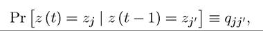

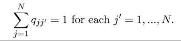
Here qjji is also referred to as a transition probability, meaning the probability of the stochastic state z transitioning from zj∣ to zj. I will make use of this notation in some of the proofs in the next section.
To see how this particular way of introducing stochastic elements into dynamic optimization is useful in economic problems, let us start with a simple example, which is also useful for introducing some additional notation.
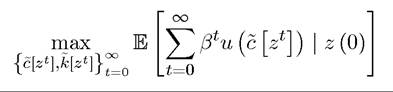
EXAMPLE 16.1. Recall the optimal growth problem, where the objective is to maximize
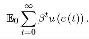
As usual, c (t) denotes per capita consumption at time t and u (∙) is the instantaneous utility function. The maximand in this problem differs from those we have seen so far only because of the presence of the expectations operator, which stands for expectations conditional on information available at time t = 0.
of consumption per capita is stochastic (as they will depend on the realization of future z’s). In particular, suppose that the production function (per capita) takes the form
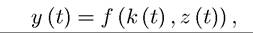
where k (t) again denotes the capital-labor ratio and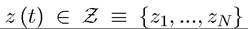 represents
a stochastic variable that affects how much output will be produced with a given amount of inputs. We continue to assume that z (t) follows a Markov chain. The most natural interpretation of z (t) in this context is as a stochastic TFP term, so one might be tempted to write y (t) = z (t) f (k (t)) and in the next chapter I will sometimes impose this form, but there is no mathematical or economic gain from doing so here. Consequently, the constraint facing the maximization problem at time t takes the form

k (t) ≥ 0 and given k (0), with δ again representing the depreciation rate. This formulation implies that at the time consumption c (t) is chosen, the random variable z (t) has been realized, thus c(t) is a random variable depending on the realization of z (t). In fact, more generally, c (t) may depend on the entire history of the random variables. For this reason, let us define
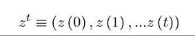
as the history of variable z (t) up to date t. Let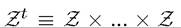 (the t-times product),
so that For given k (0), the level of consumption at time t can be most generally
written as
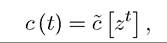
which simply states that consumption at time t will be a function of the entire sequence of random variables observed up to that point.
Clearly, consumption at time t cannot depend on future realizations of the random variable—those values have not been realized yet. Therefore, a consumption plan that depends on future realizations of the stochastic variable z would not be feasible. A function of the form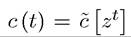 is thus natural. Nevertheless, not all
 functions could be admissible as feasible plans, because they may violate the resource constraint. We will shortly return to additional restrictions to ensure feasibility. There is also no point in making consumption a function of the history of capital stocks at this stage, since those are endogenously determined by the choice of past consumption levels and by the realization of past stochastic variables. (When we turn to the recursive formulation of this problem, we will write consumption as a function of the current capital stock and the current 615
value of the stochastic variable). Let x (t) = k (t), so that
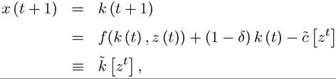
where the second line simply uses the resource constraint with equality and the third line defines the function k [zt]. With this notation, feasibility is easier to express, since  by definition depends only on the history of the stochastic shocks up to time t and not on z (t + 1). In addition, feasibility requires that the function
 satisfies

The maximization problem can then be expressed as
subject to the constraint

and starting with the initial conditions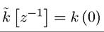 and z (0). We can also write this maxi
mization problem using the instantaneous payoff function U (x (t),x (t + 1),z (t)) introduced above.
In this case, the maximization problem would take the form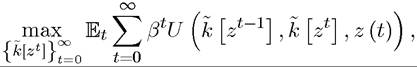
where now Notice the
timing convention here: is the value of the capital stock at time t, which is inherited
from the investments at time t — 1 and thus depends on the history of stochastic shocks up to time t — 1, zt-1, whereas is the choice of capital stock for next period made at time t given the history of stochastic shocks up to time t, zt.
This example can also be used to give us a first glimpse of how to express the same maximization problem recursively. Since z (t) follows a Markov chain, the current value of z (t) contains both the information about the available resources for consumption and future capital stock and the information regarding the stochastic distribution of z (t + 1). Thus we might naturally expect the policy function determining the capital stock at the next date to take the form

With the same reasoning, the recursive characterization would naturally take the form
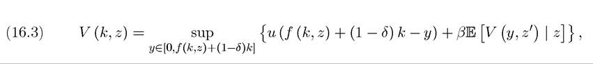
where denotes the expectation conditional on the current value of z and incorporates the fact that the random variable z is a Markov chain. Let us suppose that this program has a solution, meaning that there exists a feasible plan that achieves the value V (k, z) starting with capital-labor ratio k and stochastic variable z.
 and
and For any
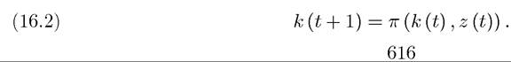

When the correspondence Π (k, z) is single valued, then π (k, z) would be uniquely defined and the optimal choice of next period’s capital stock can be represented as in (16.2).
Example 16.1 already indicates how we could write a stochastic optimization problem in a sequential form and also gives us a hint about how to express such a problem recursively. 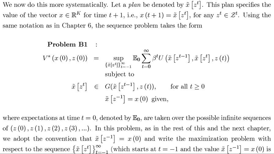 introduced as an additional constraint). The function V * is conditioned on
 , since
this is the initial value of the vector x, taken as given, and also on z (0), since the choice of x (1) is made after z (0) is observed. Finally, the first constraint in Problem B1 ensures that the sequence is feasible.
Similar to (16.3) in Example 16.1, the functional equation corresponding to the recursive formulation of this problem can be written as:
Problem B2

where V : X ? Z → R is a real-valued function and y ∈ G(x, z) represents the constraint on next period’s state vector as a function of the realization of the stochastic variable z. Problem B2 is a direct generalization of the Bellman equation in Problem A2 of Chapter 6 to a stochastic dynamic programming setup. One can also write Problem B2 as

where denotes the Lebesgue integral of the function f with respect to the
Markov process for z given last period’s value of z as z∪. This notation is useful in emphasizing that an expectation is nothing but a Lebesgue integral (and thus contains regular summation as a special case). Remembering the equivalence between expectations and integrals is important both for a proper appreciation of the theory and also for recognizing where some of the difficulties in the use of stochastic methods may lie.2 There is typically little gain in rigor or insight in using the explicit Lebesgue integral instead of the expectation and I will not do so unless absolutely necessary.
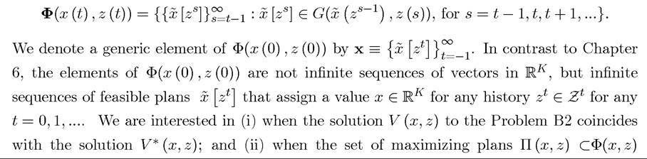
As in Chapter 6, we would like to establish conditions under which the solutions to Problems B1 and B2 coincide. Let us first introduce the set of feasible plans starting with an initial value x (t) and a value of the stochastic variable z (t) as
also generates an optimal feasible plan for Problem B1 (presuming that both problems have feasible plans attaining their supremums). Recall that the set of maximizing plans Π (x, z) is defined such that for any π (x, z) ∈ Π (x, z), we have

2
[1]In particular, potential difficulties arise when one needs to exchange limits and expectations; in contrast, there is no problem in differentiating a functional under the integral or the expectations sign as long as the integrand is differentiable.
We now introduce analogs of Assumption 6.1-6.5 from Chapter 6 and the appropriate generalizations of Theorems 6.1-6.6.
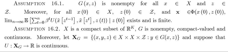
Observe that Assumption 16.1 only imposes the compactness of X, since Z is already compact in view of the fact that it consists of a finite number of elements. Moreover, the continuity of U in (x,y,z) is equivalent to its continuity in (x,y), since Z is a finite set, so we can endow it with the discrete topology, so that continuity is automatically guaranteed. As in Chapter 6, these assumptions enable us to establish a number of useful results about the equivalence between Problems B1 and B2 and the solution to the dynamic optimization problems specified above. I state these results without proof here, and provide some of the proofs in Section 16.2 and leave the rest to exercises.
Our first result is a generalization of Theorem 6.1 from Chapter 6.
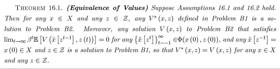
The next theorem establishes the principle of optimality for stochastic problems. As in Chapter 6, the principle of optimality enables us to break the returns from an optimal plan into two parts, the current return and the continuation return, which now corresponds to expected returns. 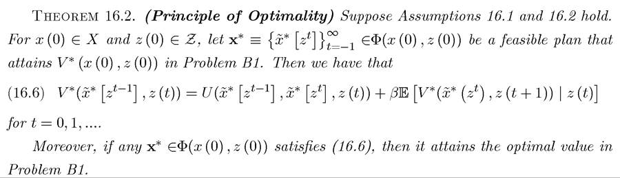
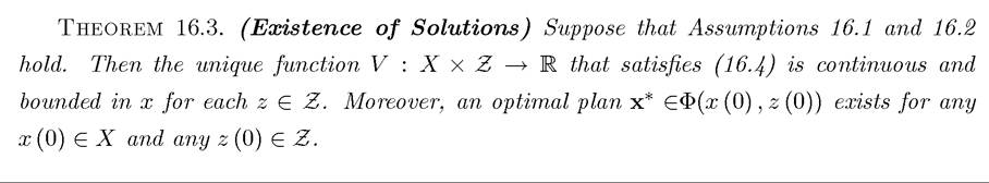
The next result establishes the uniqueness of the value function and existence of solutions.
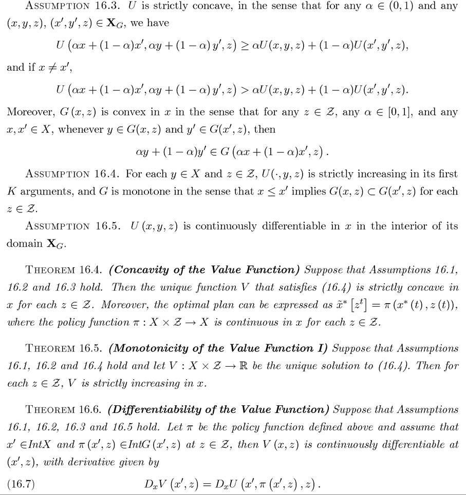
The remaining results, as their analogs in Chapter 6 use further assumptions to establish concavity, monotonicity and the differentiability of the value function.
620
These theorems have exact analogs in Chapter 6. Since the value function now also depends on the stochastic variable z, an additional monotonicity result can also be obtained. For this, let us introduce the following additional assumption: 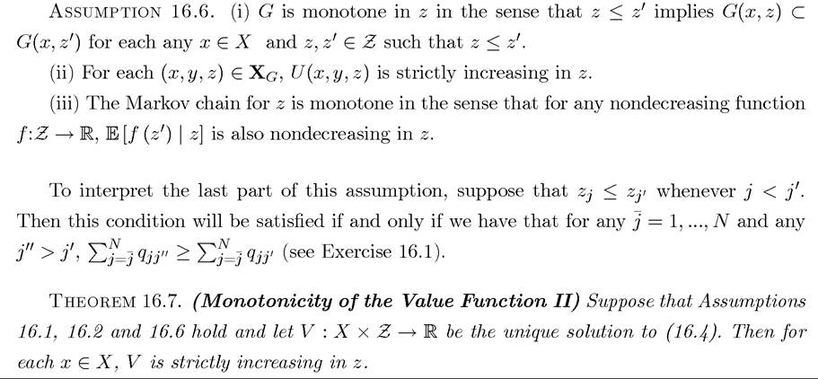
16.2.