Exercises

Exercise 7.1. Consider the problem of maximizing (7.1) subject to (7.2) and (7.3) as in Section 7.1. Suppose that for the pair (X (t),y (t)) there exists a time interval (t',t") with t' < t" such that

Prove that the pair (x (t),y (t)) could not attain the optimal value of (7.1).

Exercise 7.2. * Prove that, given in optimal solution x (t),y(t~) to (7.1), the maximized Hamiltonian defined in (7.16) and evaluated at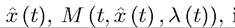is differentiable in x

and satisfies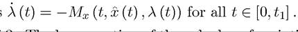

Exercise 7.3. The key equation of the calculus of variations is the Euler-Legrange equation, which characterizes the solution to the following problem (under similar regularity conditions to those of Theorem 7.2):

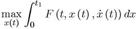
subject to X (t) = 0. Suppose that F is differentiable in all of its arguments and an interior continuously differentiable solution exists. The so-called Euler-Legrange equation, which provides the necessary conditions for an optimal solution, is

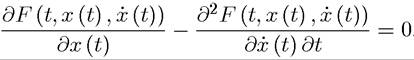
Derive this equation from Theorem 7.2. [Hint: define y (t) ? X (t)].

Exercise 7.4. This exercise asks you to use the Euler-Legrange equation derived in Exercise 7.3 to solve the canonical problem that motivated Euler and Legrange, that of finding the shortest distance between two points in a plane. In particular, consider a two dimensional plane and two points on this plane with coordinates (zo,uo) and (zι,uι). We would like to find the curve that has the shortest length that connects these two points.

conditions uo = x (zo) and uι = x (zι). It is also natural to impose that this curve u = x (z) be smooth, which corresponds to requiring that the solution be continuously differentiable so that x⁰ (z) exists.

To solve this problem, observe that the (arc) length along the curve x can be represented as

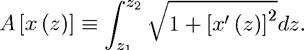
The problem is to minimize this object by choosing x (z).

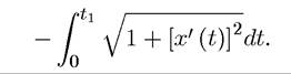
Now, without loss of any generality let us take (zo,uo) = (0, 0) and let t = z to transform the problem into a more familiar form, which becomes that of maximizing

Prove that the solution to this problem requires

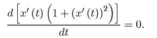
Show that this is only possible if x" (t) = 0, so that the shortest path between two points is a straight-line.

Exercise 7.5. Prove Theorem 7.2, in particular, paying attention to constructing feasible variations that ensure x (tχ,ε) = xι for all ε in some neighborhood of 0. What happens if there are no such feasible variations?

Exercise 7.6. (1) Provide an expression for the initial level of consumption c (0) as a

function of a (0), w, r and β in Example 7.1.

(2) What is the effect of an increase in a (0) on the initial level of consumption c (0)? What is the effect on the consumption path?

(3) How would the consumption path change if instead of a constant level of labor earn­ings, w, the individual faced a time-varying labor income profile given by [w (t)]1₌o? Explain the reasoning for the answer in detail.

Exercise 7.7. Prove Theorem 7.4.

Exercise 7.8. * Prove a version of Theorem 7.5 corresponding to Theorem 7.2. [Hint: instead of λ (tι) = 0, the proof should exploit the fact that x (1) = X (1) = xι].

Exercise 7.9. * Prove that in the finite-horizon problem of maximizing (7.1) or (7.11) subject to (7.2) and (7.3), f_x (t, x (t),y (t),λ (t)) > 0 for all t ∈ [0,tι] implies that λ (t) > 0 for all t ∈ [0,tι].

Exercise 7.10. * Prove Theorem 7.6.

Exercise 7.11. Prove Theorem 7.11.

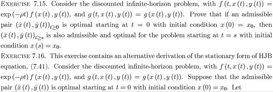
Exercise 7.12. Provide a proof of Theorem 7.15.

Exercise 7.13. Prove that in the discounted infinite-horizon optimal control problem con­sidered in Theorem 7.14 conditions (7.52)-(7.54) are necessary.

Exercise 7.14. Consider a finite horizon continuous time maximization problem, where the ob jective function is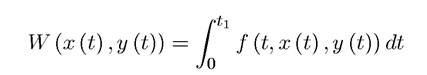

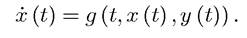
with x (0) = xo and tι < ∞, and the constraint equation is

Imagine that tχ is also a choice variable.

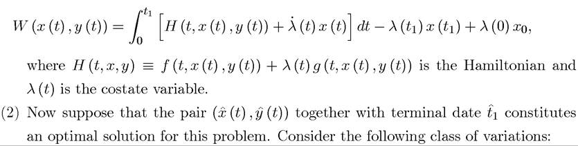
(1) Show that W (x (t),y (t)) can be written as

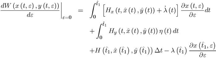
Denote the corresponding path of the state variable by x (t, ε). Evaluate W (x (t, ε),y (t, ε)) at this variation. Explain why this variation is feasible for ε small enough.

(3) Show that for a feasible variation,

(4) Explain why the previous expression has to be equal to 0.

(5) Now taking the limit as t∖ → ∞, derive the weaker form of the transversality con­dition (7.45).

(6) What are the advantages and disadvantages of this method of derivation relative to that used in the proof of Theorem 7.13.

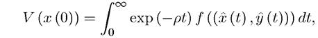
which is well defined in view of Exercise 7.15. Now write

where o (∆t) denotes second-order terms that satisfy lim∆_t→o o (∆t) /∆t = 0. Explain why

this equation can be written as

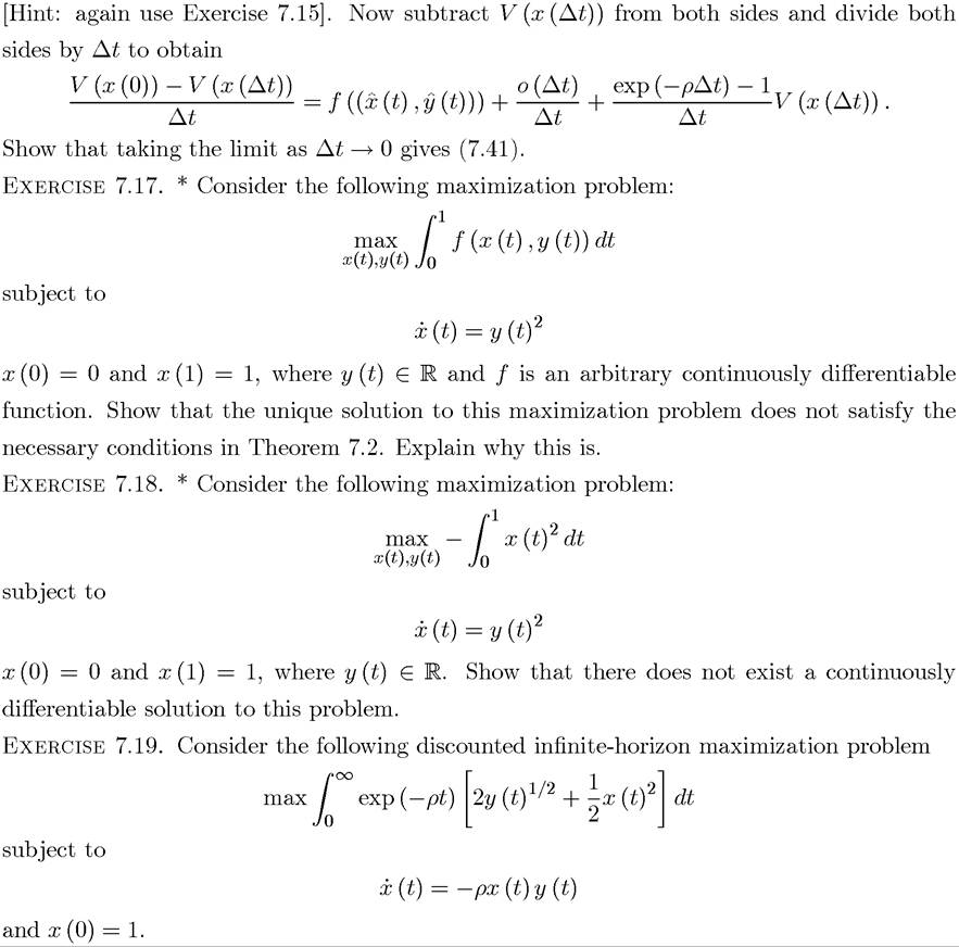
(1) Show that this problem satisfies all the assumptions of Theorem 7.14.

(2) Set up at the current-value Hamiltonian and derive the necessary conditions, with the costate variable μ (t).

(3) Show that the following is an optimal solution y (t) = 1, x (t) = exp(-ρt), and μ (t) = exp (ρt) for all t.

(4) Show that this optimal solution violates the condition that lim_t→∞ exp (—pt) μ (t), but satisfies (7.56).

Exercise 7.20. Consider the following optimal growth model without discounting:

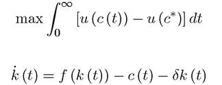
subject to

with initial condition k (0) > 0, and c* defined as the golden rule consumption level

where k* is the golden rule capital-labor ratio given by

(1) Set up the Hamiltonian for this problem with costate variable λ (t).

(2) Characterize the solution to this optimal growth program.

(3) Show that the standard transversality condition thatis not

satisfied at the optimal solution.

Exercise 7.21. Consider the infinite-horizon optimal control problem given by the maximiza­tion of (7.28) subject to (7.29) and (7.30). Suppose that the problem has a quasi-stationary structure, so that

where β (t) is the discount factor that applies to returns that are an interval of time t away from the present.

(1) Set up Hamiltonian and characterize the necessary conditions for this problem.

(2) Prove that the solution to this problem is time consistent (meaning that the solution

chosen at some date s cannot be improved upon at some future date s' by changing the continuation plans after this date) if and only iffor some ρ ≥ 0.

(3) Interpret this result and explain in what way the conclusion is different from that of Lemma 7.1.

Exercise 7.22. Consider the problem of consuming a non-renewable resource in Example

7.3. Show that the solution outlined their satisfies the stronger transversality condition (7.56).

Exercise 7.23. Consider the following continuous time discounted infinite horizon problem:

with initial condition x (0) > 0.

(1) Set up the current value Hamiltonian and derive the Euler equations for an optimal path.

(2) Show that the standard transversality condition and the Euler equations are neces­sary and sufficient for a solution.

(3) Characterize the optimal path of solutions and their limiting behavior.

Exercise 7.24. (1) In the q-theory of investment, prove that when φ" (i) = 0 (for

all i), investment jumps so that the capital stock reaches its steady-state value k* immediately.

(2) Prove that as shown in Figure 7.1, the curve for (7.64) is downward sloping in the neighborhood of the steady state.

(3) As an alternative to the diagrammatic analysis of Figure 7.1, linearize (7.61) and (7.64), and show that in the neighborhood of the steady state this system has one positive and one negative eigenvalue. Explain why this implies that optimal invest­ment plans will tend towards the stationary solution (steady state).

(4) Prove that when

(5) Derive the equations for the q-theory of investment when the adjustment cost takes

the formHow does this affect the steady-state marginal product of capital?

(6) Derive the optimal equation path when investment is irreversible, in the sense that we have the additional constraint i > 0.