Exercises
Exercise 19.1. Prove Proposition 19.1.
Exercise 19.2. Prove Proposition 19.2. [Hint: use (19.5) together with the fact that consumption and output grow at the same rate in each country to show that in the steady state it is optimal for each country (or each consumer in each country) to choose Aj (t) → 0.] Consider the world economy with free flows of capital, but assume that each country has a different discount factor ρj.
(1) Prove that 19.1 still holds.
(2) Show that there does not exist a steady-state equilibrium with Aj (t) = 0 for all j. Explain the intuition for this result.
(3) Characterize the asymptotic equilibrium (i.e., the equilibrium path as t → ∞). Suppose that ρj, < pj for all j = j0. Show that the share of the world capital that is used in country j0 will tend to 1. What does this imply for the relationship between GDP and GNP across countries.
(4) Is the form of the asymptotic equilibrium in part 3 of this exercise realistic? If not, explain how you would modify the model to achieve a more realistic world equilibrium in the presence of free capital flows.
Exercise 19.3. This exercise asks you to prove Proposition 19.3.
(1) Show that Cj (t) /cji (t) is constant for all j and j0.
(2) Show that given the result in Proposition 19.1, the integrated world equilibrium can be represented by a single aggregate production function. [Hint: use an argument similar to that leading to Proposition 19.6].
(3) Relate this result and Proposition 19.6 to Theorem 5.4 in Chapter 5. Explain why these “aggregation” results would not hold without free capital flows.
(4) Given the result in parts 1 and 2, apply an analysis similar to that for the global stability of the equilibrium path in the basic neoclassical growth model to establish the global stability of the equilibrium path here.
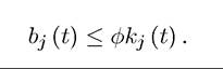
Given global stability, prove the uniqueness of the equilibrium path.Exercise 19.4. * Consider a world economy with international capital flows, but suppose that because of sovereign risk a country cannot borrow more than a fraction φ > 0 of its capital stock. Consequently, in terms of the model in Section 19.1, we have the restriction that
(1) Show that the steady-state equilibrium of the world economy is not affected by this constraint. Explain the intuition for this result carefully.
(2) Characterize the transitional dynamics of the world economy under this constraint. Show that Corollary 19.1 no longer holds.
Exercise 19.5. Barro and Sala-i-Martin (1994, 2004) use growth regressions to look at the patterns of convergence across U.S. regions and states. They find that there is a slow pattern of convergence across regions and states and they interpret this through the lenses of the neoclassical growth model. Explain why Corollary 19.1 implies that this interpretation is not appropriate. Suggest instead an alternative explanation for why convergence across regions and states might be slow. [Hint: should we expect technology or capital to flow more rapidly across regions?]
Exercise 19.6. Consider the the baseline AK model studied in Chapter 11, and suppose that countries have the same production technology, but differ according to their discount rates, the ρj's. Show that there will be persistent differences in saving and investment rates across countries that are correlated, even in the presence of free financial flows across countries. Provide a precise intuition for this result. Explain why this model could not account for the Feldstein-Horioka puzzle, which does not refer to the correlation between saving and investment in levels but in differences. Can you extend this model to account for the Feldstein- Horioka puzzle?
Exercise 19.7. Prove Proposition 19.4.
Exercise 19.8. Consider the model in Section 19.3 with different discount rates across countries. Prove that there does not exist a steady-state equilibrium.
Exercise 19.9. * Consider the model in Section 19.3, but assume that (19.9) is now modified to

where Bj's potentially differ across countries. Characterize the world equilibrium in this case. Exercise 19.10. *
(1) Show that all the results in Section 19.3 continue to hold if the constant relative risk aversion preferences in (19.14) is now modified to an arbitrary strictly increasing, strictly concave utility function u (c).
(2) Now let us go back to the preferences as in (19.14), but suppose that productivity of labor in each country is given by
Aj (t) = Aj exp (gt).
Show that all of the results from the text continue to apply, and in particular, derive the equivalent of Proposition 19.4.
(3) Finally, let us suppose that F in (19.7) does not satisfy Assumption 2. How does this affect the analysis and the results?
Exercise 19.11. Derive the unit cost functions (19.26) and (19.27) from the production functions (19.23) and (19.24). Determine the value of the constant χ.
Exercise 19.12. Derive (19.28) and (19.29).
Exercise 19.13. Consider the model in Section 19.4.
(1) Derive the trade balance equation (19.33) from the capital market clearing equation,
(19.25).
(2) Prove that the ratio of imports to GDP at each t is equal to τ.
Exercise 19.14. Provide a rigorous proof of the global stability of the steady-state world equilibrium in Proposition 19.10.
Exercise 19.15. (1) Derive (19.39) and (19.40).
(2) Explain why different parameters determine cross-country income dispersion in these
two equations.
(3) Using reasonable parameter values show how the model with international trade can generate much larger differences in income per capita across countries resulting from
small parameter differences.
Exercise 19.16. Derive equation (19.42).
Exercise 19.17. Prove Proposition 19.11.
Exercise 19.18. Prove Proposition 19.12.
Exercise 19.19. Consider the steady-state world equilibrium in the model of Section 19.4.
(1) Show that an increase in τ does not necessarily increase the steady-state world equilibrium growth rate g* as given by (19.37). Provide an intuition for this result.
(2) Show that even when τ does not increase growth, it increases world welfare. [Hint: to simplify the answer to this part of the question, you can simply look at steady state welfare].
(3) Interpret this finding in light of the debate about the effect of trade on growth.
(4) Provide a sufficient condition for an increase in τ to increase the world growth rate and interpret this condition.
Exercise 19.20. * Consider the model of Section 19.4, except that instead of utility maximization by a representative household, assume that each country saves a constant fraction Sj 803
of its income. Show that terms of trade effects will be present in equilibrium, but the steady state will be “degenerate,” with the relative prices of goods supplied by the highest saving country going to zero. Explain why exogenous savings versus dynamic utility maximization give different answers in this case.
EXERCISE 19.21. * Consider the model of Section 19.4, but assume that ε < 1. Characterize the equilibrium. Show that in this case countries that have lower discount rates will be relatively poor. Provide a precise intuition for this result. Explain why the assumption that ε < 1 may not be plausible.
Exercise 19.22. * Consider the baseline AK model in Section 19.4. Suppose that production and allocation decisions within each country is made by a “country-specific social planner” (who maximizes the utility of the representative consumer within the country).
(1) Show that the equilibrium in the text is no longer an equilibrium. Explain why.
(2) Characterize the equilibrium in this case and show that all of the qualitative results derived in the text apply. In particular, provide generalizations of Propositions 19.11 and 19.12.
(3) Show that world welfare is lower in this case than in the equilibrium in the text. Explain why.
(4) Do you find the equilibrium in this exercise or the one in the text more plausible? Justify your answer.
Exercise 19.23. * Consider the model with labor in Section 19.4. Suppose that countries can invest in order to create new varieties that they will be able to sell to the world. Suppose that if a particular firm creates such a variety, it can charge a markup equal to the monopoly price to all consumers in the world.
(1) Show that the optimal monopoly price for a firm in country j at time t is: pj (t) =
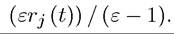 Interpret this equation.
(2) Suppose that a new variety can be created by using 1∕η units of labor. Show how this changes the labor market clearing condition and specify the free entry condition.
(3) Derive the world income distribution and show that it is stable, so that the same forces as in the model with exogenous distribution of products across countries apply in this model.
(4) What happens if new products can be produced using a combination of labor and capital?
Exercise 19.24. Show that in the model of Section 19.5 an increase in ι will always (weakly) close the relative income gap between the North and the South. Characterize the conditions under which an increase in ι will make the North worse-off (in terms of reducing its real income). Interpret these results.
Exercise 19.25. This exercise asks you to endogenize innovation decisions in the model of Section 19.5. Assume that new goods are created by technology firms in the North as in the model in Section 13.4 in Chapter 13, and these firms are monopolist suppliers until the good they have invented is copied by the South.
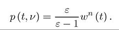
The technology of production is the same as before, and assume that new goods can be produced by using final goods, with the technology N (t) = ηZ (t), where Z (t) is final good spending. Imitation is still exogenous and takes place at the rate ι. Once a good is imitated, it can be produced competitively in the South.(1) Show that for a good that is not copied by the South, the price will be
(2) Characterize the equilibrium for given levels of Nn (t) and No (t).
(3) Compute the net present value of a new product for a Northern firm. Why does it differ from the expression in Section 13.4?
(4) Impose the free entry condition and derive the equilibrium rate of technological change for the world economy. Compute the world growth rate.
(5) What is the effect of an increase in ι on the equilibrium? Can an increase in ι make the South worse-off? Explain the intuition for this result.
Exercise 19.26. Consider a variation of the product cycle model in Section 19.5. Suppose there is no international trade, so that, the number of goods produced and consumed in each country will differ.
(1) Show that wages and incomes in the North and the South at time t are 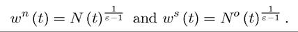
(2) Derive a condition for relative income differences to be smaller in this case than in the model with international trade. Provide a precise intuition for why international trade may increase relative income differences
(3) If trade increases the income differences between the North and the South, does it mean that it reduces welfare in the South? [Hint: if you wish, you can again use the steady-state welfare levels].
Exercise 19.27. Prove Proposition 19.13.
Exercise 19.28. Prove Proposition 19.14.
Exercise 19.29. Consider the model in Section 19.6, but assume that new products are created with the innovation possibilities frontier as in Section 13.2 in Chapter 13. Assume that before trade knowledge spillovers are created by the entire set of available inputs in the world economy, that is, the innovation possibilities frontier is similar to (13.24) in Section
13.2, except that
for country j, where is the number workers working in
R&D in country j. Consequently, trade opening does not change the structure of knowledge spillovers.
(1) Show that in this model, trade opening has no effect on the equilibrium growth rate. Provide a precise intuition for this result.
(2) Next assume that before trade opening the innovation possibly the frontier takes
the form Show that in this case, trade opening leads to an
increase in the equilibrium growth rate as in Proposition 19.14. Explain why the results are different.
(3) Which of the specifications in 1 and 2 is more plausible? In light of your answer to this question, how do you think trade opening should affect economic growth.
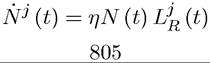
Exercise 19.30. Consider the model in Section 19.6, with two differences. First, population grows at the rate n in both countries. Second, the innovation possibilities frontier is given as  for country j, where
 Show that trade opening leads to greater
technological progress upon impact, but the long-run growth rate of each country remains unchanged.
Exercise 19.31. Prove Proposition 19.15.
Exercise 19.32. (1) Prove Proposition 19.16.
(2) Explain why when ε = 1, specialization in the sector without learning-by-doing does not have an adverse effect on the relative income of the South.
(3) What are the implications of trade opening on relative incomes if ε < 1?
(4) Characterize the equilibrium if all economies are closed until time t = T and then open to international trade at time T. What are the implications of this result for infant industry protection.
Exercise 19.33. Consider the economy in Section 19.7, but assume that the South is bigger than the North.
(1) Show that in this case not all Southern workers will work in sector 2 and there will be some learning-by-doing in the South.
(2) How does this affect the long-run equilibrium? [Hint: show that the limiting value