Exercises
Exercise 22.1. Prove that T given by (22.16) satisfies T ∈ (0,1).
Exercise 22.2. Consider the model in Section 22.2, with the only difference that the production technology is as in the Romer (1986) model studied in Chapter 11.
In particular, recall that each entrepreneur now has access to the production function Yi (t) = F (Ki (t),A (t) Li (t)) and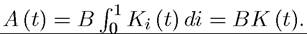 Characterize the Markov Perfect
 Political Economy Equilibrium in this case and show that distortionary taxes by the elite reduce the equilibrium growth rate of the economy.
Exercise 22.3. Consider the model in Section 22.2 and assume that policies are decided by the middle class. Show that the middle class might prefer positive taxation on themselves (with the proceeds redistributed to themselves as lump-sum transfers). Provide a precise intuition for why such taxation may make political-economic sense for middle-class entrepreneurs. Would the same result apply if the proceeds of taxation were redistributed as a lump-sum transfer to every individual in the society (including workers).
Exercise 22.4. Prove Proposition 22.4. Check in particular that the maximization program of the elite is concave, so that when T < 1 — α, the utility-maximizing tax rate for the elite is T.
Exercise 22.5. (1) Prove Proposition 22.5.
(2) Explain why the Condition 22.2 is necessary in this proposition.
(3) What happens if Condition 22.2 is not satisfied?
Exercise 22.6. Prove Proposition 22.6.
Exercise 22.7. Consider a model in Section 22.3 and suppose that the middle class are in political power. Characterize the Markov Perfect Political Economy Equilibrium in this case. Derive the discounted utility of the elite when the middle class are in control of politics, denoted by Ve (M), and compare this to their utility when they are in control, Ve (E).
[Hint: see Section 23.2 in the next chapter and Exercise 23.2].Exercise 22.8. In the model with political replacement in subsection 22.3.2, suppose that η' (∙) < 0. Show that in this case the tax rate preferred by the elite is less than 1 — α and that when the elite can block technology adoption, they will not choose to do so. Explain the intuition for this result. What types of institutional structures might lead to η0 (∙) < 0 as opposed to η0 (∙) > 0.
Exercise 22.9. Prove Proposition 22.7.
Exercise 22.10. In the model with political replacement in subsection 22.3.2, show that the unique MPE is also the unique SPE.
Exercise 22.11. (1) Prove Proposition 22.9.
(2) Explain how Proposition 22.9 needs to be modified if τ < 1 and provide an analysis of the best stationary SPE in this case.
Exercise 22.12. Prove Proposition 22.13.
Exercise 22.13. Prove Proposition 22.14.
Exercise 22.14. Prove Proposition 22.16. Exercise 22.15. (1) Prove Proposition 22.17.
(2) Now suppose that in this proposition φ is not equal to 0. Provide an example in which in the MPE, the elite would still prefer g = 0.
(3) Now suppose that the elite can charge lump-sum taxes to middle-class entrepreneurs. Provide an example in which in the MPE, the elite would still prefer g = 0.
(4) In light of your answers to 2 and 3 above, explain why the political equilibrium might involve the use of inefficient fiscal instruments, even when more efficient alternatives
exist.
Exercise 22.16. * Prove Proposition 22.18.
Exercise 22.17. * Prove Proposition 22.19.
Exercise 22.18. Consider an environment with concave preferences as in Section 22.5. Assume that there is full depreciation (i.e., δ = 1), citizens are yeoman-producers only using their own labor and have access to a production technology for producing the unique final good given by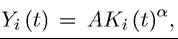 where Ki (t) is the capital holding of producer i.
citizens and elites have logarithmic preferences. Characterize the MPE in this environment. [Hint: conjecture a policy rule that depends only on the current (average) net output, so that the tax rate for next period is where K (t) is the common capital stock of all producers].
Exercise 22.19. * Prove that if individual preferences are reflexive, complete and transitive, then they can be represented by a real-valued utility function.
Exercise 22.20. *
(1) Consider a society with two individuals 1 and 2 and three choices, a, b and c. For the purposes of this exercise, only consider strict individual and social orderings (i.e., no indifference allowed). Suppose that the preferences of the first agent are given by abc (short for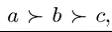 i.e., a strictly preferred to b, strictly preferred to c).
Consider the six possible preference orderings of the second individual, i.e., s2 ∈ {abc, acb, bac,...}, etc.. Define a social ordering as a mapping from the preferences of the second agent (given the preferences of the first) into a social ranking of the three outcomes, i.e., some function φ such that the social ranking is s = φ (s2). Illustrate the Arrow impossibility theorem using this example [Hint: start as follows: abc = φ (abc), i.e., when the second agent’s ordering is abc, the social ranking must be abc; next, φ (acb) = abc or acb (why?); then if φ (acb) = abc, we must also have
φ (cab) = abc (why?); and proceeding this way to show that the social ordering is either dictatorial or it violates one of the axioms].
(2) Now suppose we have the following aggregation rule: individual 1 will (sincerely) rank the three outcomes, his first choice will get 6 votes, the second 3 votes, the third 1 vote. Individual 2 will do the same, his first choice will get 8 votes, the second 4 votes, and the third 0 vote.
The three choices are ranked according to the total number of votes. Which of the axioms of the Arrow’s Theorem does this aggregation rule violate?(3) With the above voting rule, show that for a certain configuration of preferences, either agent has an incentive to distort his true ranking (i.e., not vote sincerely).
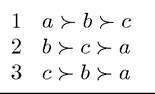
(4) Now consider a society consisting of three individuals, with preferences given by:
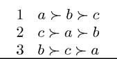
Consider a series of pairwise votes between the alternatives. Show that when agents vote sincerely, the resulting social ordering will be “intransitive”. Relate this to the Theorem 22.1.
(5) Show that if the preferences of the second agent are changed t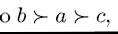 the social
ordering is no longer intransitive. Relate this to “single-peaked preferences”.
(6) Explain intuitively why single-peaked preferences are sufficient to ensure that there will not be intransitive social orderings. How does this relate to Theorem 22.1?
EXERCISE 22.21. * In the Condorcet paradox example provided in Section 22.6, show that other orderings of the choices a, b and c will also imply that the preferences of at least one of the three individuals is not single peaked.
Exercise 22.22. *
(1) Consider the example of a three-person three-policy society with preferences
Voting is dynamic: first, there is a vote between a and b. Then, the winner goes against c, and the winner of this contest is the social choice. Find the subgame perfect Nash equilibrium voting strategy profiles in this two-stage game (recall that each player’s strategy has to specify how they will vote in the first round, and how they will vote in the second round as a function of the outcome of the first round).
(2) Suppose a generalization whereby the society H consists of H individuals and there
are finite number of policies,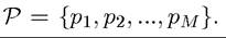 For simplicity, suppose that H
is an odd number.
Voting takes M — 1 stages. In the first stage, there is a vote1016
between pi and p2. In the second stage, there is a vote between the winner of the first stage and p3, until we have a final vote against đě. The winner of the final vote is the policy choice of the society. Prove that if preferences of all agents are single peaked (with a unique bliss point for each), then the unique subgame perfect Nash equilibrium implements the bliss point of the median voter.
Exercise 22.23. * Prove Theorem 22.2 when H is even.
Exercise 22.24. * Characterize the subgame perfect equilibrium of the game in Example 22.2 under strategic voting by all players.
Exercise 22.25. * Modify and prove Theorem 22.4 without Assumption A4.
Exercise 22.26. * This exercise reviews Downsian party competition and then show that Theorem 22.4 does not apply if there are three parties competing. In particular, consider Downsian party competition in a society consisting of a continuum 1 of individuals with single-peaked preferences. The policy space P is the [0,1] interval and assume that the bliss points of the individuals are uniformly distributed over this space.
(1) To start with, suppose that there are two parties, A and B. They both would like to maximize the probability of coming to power. The game involves both parties simultaneously announcing pA ∈ [0,1] and pB ∈ [0,1], and then voters voting for one of the two parties. The platform of the party with most votes gets implemented. Determine the equilibrium of this game. How would the result be different if the parties maximized their vote share rather than the probability of coming to power?
(2) Now assume that there are three parties, simultaneously announcing their policies pA ∈ [0,1], pB ∈ [0,1], and pc ∈ [0,1], and the platform of the party with most votes is implemented. Assume that parties maximize the probability of coming to power.
Characterize all pure strategy equilibria.(3) Now assume that the three parties maximize their vote shares. Prove that there exists no pure strategy equilibrium.
(4) In 3, characterize the mixed strategy equilibrium. [Hint: assume the same symmetric probability distribution for two parties, and make sure that given these distributions, the third party is indifferent over all policies in the support of the distribution].
Exercise 22.27. * Prove Theorem 22.6.
Exercise 22.28. * This exercise involves generalizing the idea of single-crossing property used in Theorem 22.5 to multi-dimensional policy spaces. The appropriate notion of preferences of individuals turns out to be “intermediate preferences”. Let P C R1, where I is an integer, and policies p belong to P. We say that voters have intermediate preferences, if their indirect utility function U (p; α⅛) can be written as

1017
where K(αi) is monotonic (monotonically increasing or monotonically decreasing) in α⅛, and the functions Jι(p) and J2 (p) are common to all voters. Suppose that A2 holds and voters have intermediate preferences. We define the bliss point (vector) of individual i as in the text, as p (αi) ∈ P that maximizes individual i’s utility. Prove that when preferences are intermediate a Condorcet winner always exists and coincides with bliss point of the voter with the median value of αγ that is, pm = p (αm).
Exercise 22.29. * Consider a society consisting of three individuals, 1, 2 and 3 and a resource of size 1. The three individuals vote over how to distribute the resource among themselves and each individual prefers more of the resource for himself and does not care about consumption by the other two. Since all of the resource will be distributed among the three individuals, we can represent the menu of policies as {(x1,x2) : χι ≥ 0, χ2 ≥ 0 and xι + x2 ≤ 1}, where Xi denotes the share of the resource consumed by individual i. A policy vector (x1,x2) is accepted if it receives two votes.
(1) Show that individual preferences over policy vectors do not satisfy single crossing or the conditions in Exercise 22.28.
(2) Show that there does not exist a policy vector that it is a Condorcet winner.
Exercise 22.30. *
(1) Show that in Theorem 22.7, a necessary condition for a pure strategy symmetric equilibrium, with pa = đâ = p*, to exist is that the matrix
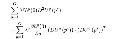
is negative semidefinite, where D2Ug denotes the Jacobian matrix of Ug.
(2) Derive a sufficient condition for such a symmetric equilibrium to exist. [Hint: distinguish between local and global maxima].
(3) Show that without any assumptions on Ug (∙)'s (beyond concavity), the sufficient condition for a symmetric equilibrium can only be satisfied if all Hg's are uniform.
Exercise 22.31. Consider the following one-period economy populated by a mass 1 of agents. A fraction λ of these agents are capitalists, each owning capital k. The remainder have only human capital, with human capital distribution μ(h). Output is produced in competitive markets, with aggregate production function
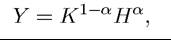
where uppercase letters denote total supplies. Assume that factor markets are competitive and denote the market clearing rental price of capital by r and that of human capital by w.
1018
(1) Suppose that agents vote over a linear income tax, τ. Because of tax distortions, total tax revenue is
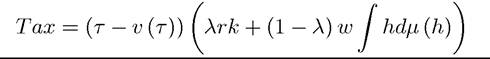
where v (τ) is strictly increasing and convex, with v (0) = v0 (0) = 0 and v0 (1) = ∞ (why are these conditions useful?). Tax revenues are redistributed lump sum. Find
the ideal tax rate for each agent. Find conditions under which preferences are single
peaked, and determine the equilibrium tax rate. How does the equilibrium tax rate change when k increases? How does it change when λ increases? Explain the intuition for these results.
(2) Suppose now that agents vote over capital and labor income taxes, τ⅛ and τh, with corresponding costs v and v
and v l so that tax revenues are
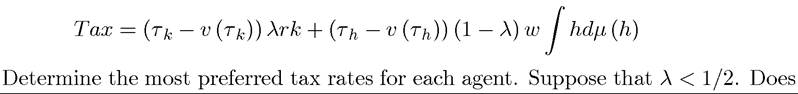
a voting equilibrium exist? Explain. How does it change when λ increases? Explain
why this would be different from the case with only one tax instrument?
(3) In this model with two taxes, now suppose that agents first vote over the capital income tax, and then taking the capital income tax as given, they vote on the labor
income tax. Does a voting equilibrium exist? Explain. If an equilibrium exists, how
does the equilibrium tax rate change when k increases? How does it change when λ
increases?
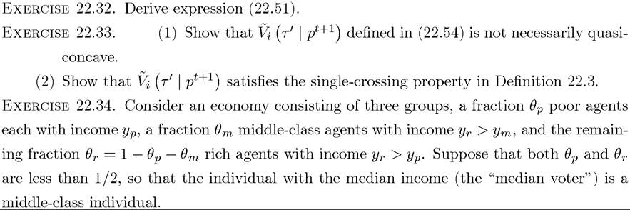
(1) Construct a change in incomes that leaves mean income in the society unchanged and increases the gap between the mean and the median but does not constitute a mean preserving spread of the distribution.
(2) Construct a mean preserving spread of the distribution such that the gap between the mean and the median narrows. [Hint: increase ym and reduce yp, holding yr constant].
Exercise 22.35. We now consider the model by Alesina and Rodrik, which is similar to the model studied in Section 22.7. There is a continuum 1 of individuals. All individuals have logarithmic instantaneous utility, so that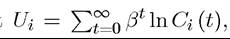 where i denotes the
individual and Ci (t) refers to his consumption at time t. Each individual has one unit of labor, which he supplies inelastically. Final output is produced as
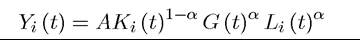
where Ki and Li denote capital and labor employed by individual i and G is government investment in infrastructure. The only tax instrument is a linear tax on the capital holdings of all individuals at the rate τ (t) at time t. All the proceeds of this taxation are spent on government investment in infrastructure, so that

where K (t) is the average (total) capital stock in the economy. This specification implies that government’s provision of infrastructure creates a Romer-type externality. Denote the initial capital stock of the economy by
(1) Characterize the equilibrium with a constant tax rate τ > 0 at each date and show that with A sufficiently large, the economy will achieve a constant and positive growth rate. Show that the growth rate of the economy is independent of the distribution of the initial capital stock among the individuals. [Hint: note that the net interest rate faced by consumers is equal to the marginal product of capital minus the tax rate, τ].
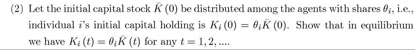
(3) Suppose that the economy will legislate a constant tax rate τ forever. Determine the most preferred tax rate of individual i as a function of his share of initial capital θi at time t = 0.
(4) Show that individuals have single-peaked preferences. On the basis of this, appeal to Theorems 22.2 and 22.4 to argue that the tax rate most preferred by the individual with the median capital holdings, θm, will be implemented. Show that as this median capital holdings falls, the rate of capital taxation increases. What is the effect of this on economic growth?
(5) Show that the equilibrium characterized in 4 above is not a Markov Perfect Political Economy Equilibrium. Explain why not. How would you set up the problem to characterize such an equilibrium? [Hint: just describe how you would set up the problem; no need to solve for the equilibrium].
Exercise 22.36. (1) Prove Proposition 22.24.
(2) Derive the output-maximizing tax rate as in (22.69).
(3) Characterize the tax rates maximizing the utility of the elite and the citizens and establish the results in Proposition 22.25.