Exercises

EXERCISE 2.1. Show that competitive labor markets and Assumption 1 imply that the wage rate must be strictly positive and thus (2.4) implies (2.3).

Exercise 2.2. Prove that Assumption 1 implies that F (A, K, L) is concave in K and L, but not strictly so.

Exercise 2.3. Show that when F exhibits constant returns to scale and factor markets are competitive, the maximization problem in (2.5) either has no solution (the firm can make infinite profits), a unique solution K = L = 0, or a continuum of solutions (that is, any (K, L) with K/L = κ for some κ. > 0 is a solution).

Exercise 2.4. Consider the Solow growth model in continuous time with the following per capita production function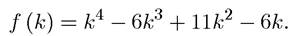

(1) Which parts of Assumptions 1 and 2 does the underlying production function F (K, L) violate?

(2) Show that with this production function, there exist three steady-state equilibria.

(3) Prove that two of these steady-state equilibria are locally stable, while one of them is locally unstable. Can any of these steady-state equilibria be globally stable?

Exercise 2.5. Prove Proposition 2.7.

Exercise 2.6. Prove Proposition 2.8.

Exercise 2.7. Let us introduce government spending in the basic Solow model. Consider the basic model without technological change. In particular, suppose that (2.9) takes the form

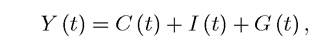
with G (t) denoting government spending at time t. Imagine that government spending is given by G (t) = σY (t).

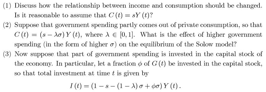
Show that if φ is sufficiently high, the steady-state level of capital-labor ratio will increase as a result of higher government spending (corresponding to higher σ).

Exercise 2.8. Suppose that F (A,K,L) is concave in K and L (though not necessarily strictly so) and satisfies Assumption 2. Prove Propositions 2.2 and 2.5. How do we need to modify Proposition 2.6?

Exercise 2.9. Prove Proposition 2.6.

Exercise 2.10. Prove Corollary 2.2.

Exercise 2.11. Recall the definition of the elasticity of substitution σ in (2.37). Suppose labor markets are competitive and the wage rate is equal to w. Prove that if the aggregate production function F (K, L, A) exhibits constant returns to scale in K and L, then

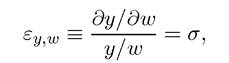
where, as usual, y ? F (K, L, A) /L.

Exercise 2.12. Consider a modified version of the continuous-time Solow growth model where the aggregate production function is

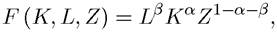
where Z is land, available in fixed inelastic supply. Assume that α + β < 1, capital depreciates at the rate δ, and there is an exogenous saving rate of s.

(1) First suppose that there is no population growth. Find the steady-state capital­labor ratio in the steady-state output level. Prove that the steady state is unique and globally stable.

(2) Now suppose that there is population growth at the rate n, that is,What

happens to the capital-labor ratio and output level as t → ∞? What happens to returns to land and the wage rate as t → ∞?

(3) Would you expect the population growth rate n or the saving rate s to change over time in this economy? If so, how?

Exercise 2.13. Consider the continuous-time Solow model without technological progress and with constant rate of population growth equal to n. Suppose that the production function satisfies Assumptions 1 and 2.

(1) Define and characterize the steady-state equilibrium of this economy and study its stability.

(2) What is the relationship between the steady-state capital-labor ratio k* and the

golden rule capital stockdefined above?

Exercise 2.14. Consider the Solow growth model with constant saving rate s and depre­ciation rate of capital equal to δ. Assume that population is constant and the aggregate production function is given by the constant returns to scale production function

(1) Suppose that F is Cobb-Douglas. Determine the steady-state growth rate and the adjustment of the economy to the steady state.

(2) Suppose that F is not Cobb-Douglas (even asymptotically). Prove that there does not exist a steady state. Explain why this is.

(3) For the case in which F is not Cobb-Douglas, determine what happens to the capital­labor ratio and output per capita as t → ∞.

EXERCISE 2.15. Consider the Solow model with non-competitive labor markets. In particular, suppose that there is no population growth and no technological progress and that output is given by F (K, L). The saving rate is equal to s and the depreciation rate is given by δ.

(1) First suppose that there is a minimum wage w, such that workers are not allowed to be paid less than w. If labor demand at this wage falls short of L, employment is equal to the amount of labor demanded by firms, L^d (and the unemployed do not contribute to production and earn zero). Assume that

where k* is the steady-state capital-labor ratio of the basic Solow model given by Characterize the dynamic equilibrium path of this economy start­ing with some amount of physical capital K (0) > 0.

(2) Next consider a different form of labor market imperfection, whereby workers receive a fraction β > 0 of output in each firm as their wage income. Characterize a dynamic equilibrium path in this case. [Hint: recall that the saving rate is still equal to s].

Exercise 2.16. Consider the discrete-time Solow growth model with constant population growth at the rate n, no technological change, constant depreciation rate of δ and a constant saving rate s. Assume that the per capita production function is given by the following continuous but non-neoclassical function:

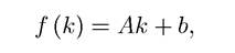
where A > 0 and b > 0.

(1) Explain why this production function is non-neoclassical (that is, why does it violate Assumptions 1 and 2 above?).

(2) Suppose that sA — n — δ = —1 (which is possible if n is sufficiently large). Show that for any k (0) ∈ (0,sb), the economy settles into an asymptotic cycle and continuously fluctuates between k (0) and sb — k (0).

(3) Now consider a more general continuous production function f (k) that does not satisfy Assumptions 1 and 2, such that there exist k1,k2 ∈ R∣ withand

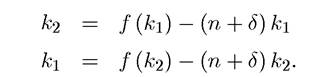
Show that when such (k1,k2) exist, there may also exist a stable steady state.

(4) Prove that such cycles are not possible in the continuous-time Solow growth model for any (possibly non-neoclassical) continuous production function f (k). [Hint: con­sider the equivalent of Figure 2.9 above].

(5) What does the result in parts 2 and 3 imply for the approximations of discrete time by continuous time suggested in Section 2.4?

(6) In light of your answer to part 5, what do you think of the cycles in parts 2 and 3? Exercise 2.17. Characterize the asymptotic equilibrium of the modified Solow/AK model mentioned above, with a constant saving rate s, depreciation rate δ, no population growth and an aggregate production function of the form

Exercise 2.18.

(1) Determine conditions under which this production function satisfies Assumptions 1 and 2.

(2) Characterize the unique steady-state equilibrium when Assumptions 1 and 2 hold.

(3) Now suppose that σ is sufficiently high so that Assumption 2 does not hold. Show that in this case equilibrium behavior can be similar to that in Exercise 2.17 with sustained growth in the long run. Interpret this result.

(4) Now suppose that σ → 0, so that the production function becomes Leontief,

The model is then identical to the classical Harrod-Domar growth model developed by Roy Harrod and Evsey Domar (Harrod, 1939, Domar, 1946). Show that in this case there is typically no steady-state equilibrium with full employment and no idle capital. What happens to factor prices in these cases? Explain why this case is “pathological,” giving at least two reasons why we may expect equilibria with idle capital or idle labor not to apply in practice.

Exercise 2.19. * We now derive the CES production function following the method in the original article by Arrow, Chenery, Minhas and Solow (1961). These authors noted that a good empirical approximation to the relationship between income per capita and the wage rate was provided by an equation of the form

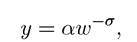
where y = f (k) is again output per capita and w is the wage rate. With competitive markets, recall that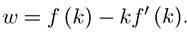Thus the above equation can be written as

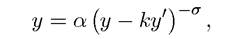
where y = y (k) ? f (k) and y' denotesThis is a nonlinear first-order differential equation.

(1) Using separation of variables (see Appendix Chapter B), show that the solution to this equation satisfies

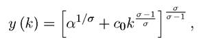
where co is a constant of integration.

81

(2) How would you put more structure on α and co and derive the exact form of the CES production function in (2.38)?

Exercise 2.20. Show that the see as production function with σ > 1 violates Assumption 1 and with σ ≤ 1, it satisfies Assumption 1.

Exercise 2.21. Prove Proposition 2.12.

Exercise 2.22. Prove Proposition 2.13.

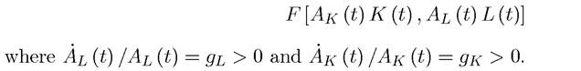
Exercise 2.23. In this exercise, we work through an alternative conception of technology, which will be useful in the next chapter. Consider the basic Solow model in continuous time and suppose that A (t) = A, so that there is no technological progress of the usual kind. However, assume that the relationship between investment and capital accumulation is modified to whereis an exogenously given time-varying process. Intuitively, when q (t) is high, the same investment expenditure translates into a greater increase in the capital stock. There­fore, we can think of q (t) as the inverse of the relative prices of machinery to output. When q (t) is high, machinery is relatively cheaper. Gordon (1990) documented that the relative prices of durable machinery has been declining relative to output throughout the postwar era. This is quite plausible, especially given our recent experience with the decline in the relative price of computer hardware and software. Thus we may want to suppose that q (t) > 0. This exercise asks you to work through a model with this feature based on Greenwood, Hercowitz and Krusell (1997).

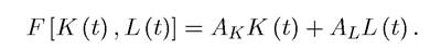
(1) Suppose that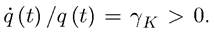Show that for a general production function,

F (K,L), there exists no steady-state equilibrium.

(2) Now suppose that the production function is Cobb-Douglas,

and characterize the unique steady-state equilibrium.

(3) Show that this steady-state equilibrium does not satisfy the Kaldor fact of constant K/Y. Is this a problem? [Hint: how is “K” measured in practice? How is it measured in this model?].

82