Exercises
Exercise 8.1. Consider the consumption allocation decision of an infinitely-lived household with (a continuum of) L (t) members at time t, with L (0) = 1. Suppose that the household has total consumption C (t) to allocate at time t.
The household has “utilitarian” preferences with instantaneous utility function u (c) and discount the future at the rate p > 0.(1) Show that the problem of the household can be written as
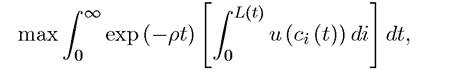
subject to
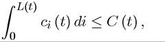
and subject to the budget constraint of
A (t) = r (t) A (t) + W (t) — C (t),
where i denotes a generic member of the household, A (t) is the total asset holding of the household, r (t) is the rate of return on assets and W (t) is total labor income.
(2) Show that as long as u (∙) is strictly concave, this problem becomes

where w (t) ? W (t) /L (t) and a (t) ? A (t) /L (t). Provide an intuition for this transformed problem.
Exercise 8.2. Consider the maximization of (8.3) subject to (8.8) without any other constraints.
(1) Show that for any candidate consumption plan there exists another consumption plar
 that satisfies the flow budget constraint (8.8), involves
c0 (t) > c (t) and yields strictly higher utility.
(2) Using the argument in part 1, show that the household will choose asset levels a (t) becoming arbitrarily negative for all t. [Hint: this problem does not have a sequence of consumption and asset levels that reach the maximum value of the objective function; so here you should simply show that a (t) arbitrarily negative for all t approaches the maximum value of the objective function (which may be, but does not need to be, +∞)].
(3) Explain why an allocation with these features would violate feasibility.
Exercise 8.3. Start with the law of motion of the total assets of the households, given by
(8.7). Using this, show that if the household starts with A (t) = 0 at time t and chooses zero consumption thereafter, then it will asymptotically generate asset holdings of
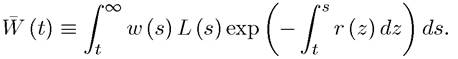
Explain why the natural debt limit requires that A (t) ≥ — IV (t). Using the definition of A (t) and the fact that L (t) grows at the rate n, derive (8.11). Relate this natural debt limit to its discrete-time analog, (6.41) in Chapter 6.
Exercise 8.4. Show that the relaxed natural debt limit (8.12) implies that the original debt limit (8.11) holds for all t.
Exercise 8.5. Derive (8.8) from (8.13).
Exercise 8.6. Derive (8.15) from (8.14) and (8.18). [Hint: use (8.17) to substitute for μ (t) in (8.18).
Exercise 8.7. Verify that Theorem 7.13 can be applied to the household maximization
and there is population growth at the constant rate n. How does this affect the equilibrium? How does the transversality condition need to be modified? What is the relationship between the rate of population growth, n, and the steady-state capital labor ratio k*?
Exercise 8.14. Prove Proposition 8.3.
Exercise 8.15. Explain why the steady state capital-labor ratio k* does not depend on the form of the utility function without technological progress, but depends on the intertemporal elasticity of substitution when there is positive technological progress.
Exercise 8.16. (1) Show that the steady-state saving rate s* defined in (8.36) is de
creasing in ρ, so that lower discount rates lead to higher steady-state savings.
(2) Show that in contrast to the Solow model, the saving rate s* can never be so high that a decline in savings (or an increase in ρ) can raise the steady-state level of consumption per capita.
Exercise 8.17. In the dynamics of the basic neoclassical growth model, depicted in Figure 8.1, prove that the c =O locus intersects the locus always to the left of kgθid. Based on this analysis, explain why the modified golden rule capital-labor ratio, k*, given by (8.34) differs from kgθid.
Exercise 8.18. Consider the neoclassical model with technological progress studied in Section 8.7. Show that when Assumption 4 is satisfied, the household maximization problem, that of maximizing (8.47) subject to (8.8) and (8.14) satisfies the sufficiency conditions in Theorem 7.14. What happens if Assumption 4 is not satisfied?
Exercise 8.19. Prove that, as stated in Proposition 8.7, in the neoclassical model with laboraugmenting technological change and the standard assumptions, starting with k (0) > 0, there exists a unique equilibrium path where normalized consumption and capital-labor ratio monotonically converge to the BGP. [Hint: use Figure 8.1].
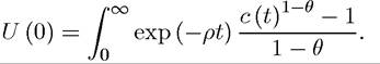
Exercise 8.20. Consider a neoclassical economy, with a representative household with preferences at time t = 0:
There is no population growth and labor is supplied inelastically. Assume that the aggregate production function is given by Y (t) = F [A (t) K(t),L (t)] where F satisfies the standard assumptions (constant returns to scale, differentiability, Inada conditions).
(1) Define a competitive equilibrium for this economy.
(2) Suppose that A (t) = A (0) for all t and characterize the steady-state equilibrium. Explain why the steady-state capital-labor ratio is independent of θ.
(3) Now assume that A (t) = exp(gt) A (0), and show that a BGP (with constant
capital share in national income and constant and equal rates of growth of output, capital and consumption) exists only if F takes the Cobb-Douglas form,
Y (¢) = (A (t) K(t))α (L (t))1-α.
(4) Characterize the BGP in the Cobb-Douglas case. Derive the common growth rate
of output, capital and consumption. Explain why the (normalized) steady-state capital-labor ratio now depends on θ.
Exercise 8.21. Consider the baseline neoclassical model with no technological progress.
(1) Show that in the neighborhood of the steady state k*, the law of motion of k (t) ?
K (t) /L (t) can be written as

where ξ1 and ξ2 are the eigenvalues of the linearized system.
(2) Compute these eigenvalues show that one of them, say ξ2, is positive.
(3) What does this imply about the value
(4) How is the value of η1 determined?
(5) What determines the speed of adjustment of k (t) towards its steady-state value k*? Exercise 8.22. Derive closed-form equations for the solution to the differential equations of transitional dynamics presented in Example 8.2 with log preferences.
Exercise 8.23. Derive eq. (8.40) from the T — 1-period lifetime budget constraint of the representative household. In particular, write this budget constraint as
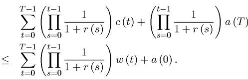
Explain why this is the correct form of the budget constraint.
By taking the limit as T → ∞, show that this constraint will imply the infinite-horizon lifetime budget constraint only if (8.40) is satisfied.
Exercise 8.24.
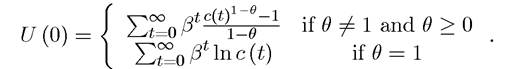
Consider the discrete-time version of the neoclassical growth model. Suppose that the economy admits a representative household with log preferences (θ = 1 in terms of(8.47) ) and the production function is Cobb-Douglas. Assume also that δ = 1,so that there is full depreciation. Characterize the steady-state equilibrium and derive a difference equation that explicitly characterizes the behavior of capital stock away from the steady state.
Exercise 8.25. Again in the discrete-time version of the neoclassical growth model, suppose that there is labor-augmenting technological progress at the rate g,
A(t +1) = (1 + g) A (t) ∙
For simplicity, suppose that there is no population growth.
(1) Prove that balanced growth requires preferences to take the CRRA form
(2) Assuming this form of preferences, prove that there exists a unique steady-state equilibrium in which effective capital-labor ratio remains constant.
(3) Prove that this steady-state equilibrium is globally stable and convergence to this steady-state starting from a non-steady-state level of effective capital-labor ratio is
monotonic.
Exercise 8.26. (1) Analyze the comparative dynamics of the basic model in response
to unanticipated increase in the rate of labor-augmenting technological progress will increase to Does consumption increase or decrease upon impact?
(2) Analyze the comparative dynamics in response to the announcement at time T that at some future date the tax rate will decline to
 Does consumption increase or decrease at time T.
Exercise 8.27. Consider the basic neoclassical growth model with technological change and CRRA preferences (8.47). Explain why θ > 1 ensures that the transversality condition is always satisfied.
Exercise 8.28. Consider the basic neoclassical growth model with CRRA preferences, but with consumer heterogeneity in initial asset holdings (you may assume no technological change if you wish). In particular, there is a set H of household and household h ∈ H starts with initial assets ¾ (0). Households are otherwise identical.
(1) Characterize the competitive equilibrium of this economy and show that it is identi
cal to the corresponding representative household economy, with the representative household starting with assets is the measure
(number) of households in this economy. Interpret this result and relate it to the aggregation theorems discussed in Chapter 5.
(2) Show that if, instead of the natural debt limit or the no-Ponzi condition, we impose
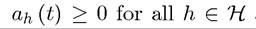 and for all t, then a different equilibrium allocation may result. In light of this finding, interpret the appropriability of using the no-borrowing constraint instead of the natural debt limit.
Exercise 8.29. Consider a variant of the neoclassical economy with preferences given by
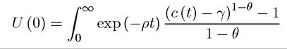
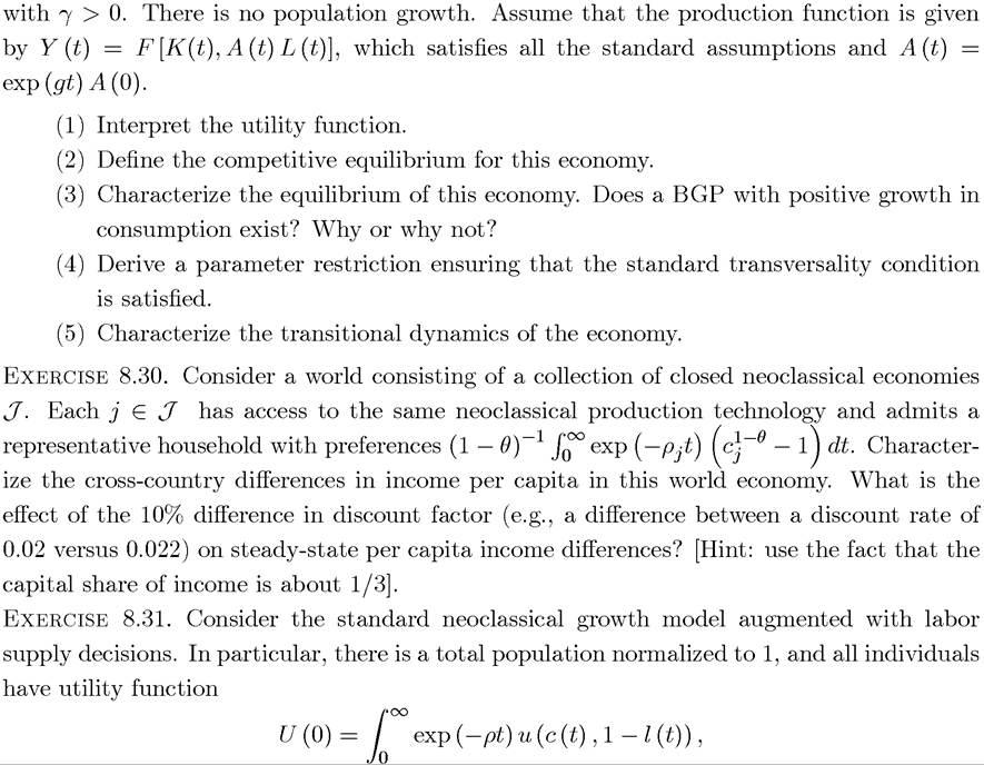
where l (t) ∈ (0,1) is labor supply. In a symmetric equilibrium, employment L (t) is equal to l (t). Assume that the production function is given by Y (t) = F [K(t),A (t) L (t)], which satisfies all the standard assumptions and A (t) = exp (gt) A (0).
(1) Define a competitive equilibrium.
(2) Set up the current-value Hamiltonian that each household solves taking wages and interest rates as given, and determine first-order conditions for the allocation of consumption over time and leisure-labor trade off.
(3) Set up the current-value Hamiltonian for a planner maximizing the utility of the representative household, and derive the necessary conditions for an optimal solution.
(4) Show that the two problems are equivalent given competitive markets.
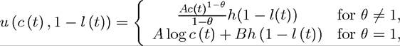
(5) Show that unless the utility function is asymptotically equal to
where G (t) is a public good financed by government spending. Assume that the production function is given by Y (t) = F [K(t),L (t)], which satisfies all the standard assumptions, and the budget set of the representative household is C (t) + I (t) ≤ Y (t), where I (t) is private investment. Assume that G (t) is financed by taxes on investment. In particular, the capital accumulation equation is
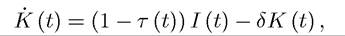
and the fraction τ (t) of the private investment I (t) is used to finance the public good, that is, G (t) = τ (t) I (t).
Take the process of tax ratesid="Picutre 1021" class="lazyload" data-src="/files/uch_group77/uch_pgroup317/uch_uch7365/image/image1020.jpg">
(1) Define a competitive equilibrium.
(2) Set up the individual maximization problem and characterize consumption and investment behavior.
(3) Assuming that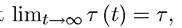 characterize the steady state.
(4) What value of τ maximizes the steady-state utility of the representative household. Starting away from the state state, is this also the tax rate that would maximize the initial utility level? Why or why not?
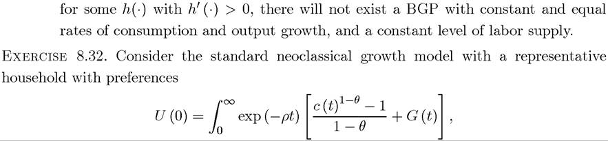
EXERCISE 8.33. Consider the neoclassical growth model with a government that needs to finance a flow expenditure of G. Suppose that government spending does not affect utility and that the government can finance this expenditure by using lump-sum taxes (that is, some amount T (t) imposed on each household at time t regardless of their income level and capital holdings) and debt, so that the government budget constraint takes the form 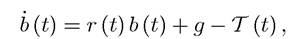
where b (t) denotes its debt level. The no-Ponzi condition for the government is
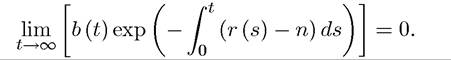
Prove the following Ricardian equivalence result: any process of lump-sum taxes that satisfy the government’s budget constraint (together with the no-Ponzi condition) leads to the same equilibrium process of capital-labor ratio and consumption. Interpret this result. Exercise 8.34. Consider the baseline neoclassical growth model with no population growth and no technological change, and preferences given by the standard CRRA utility function (8.47). Assume, however, that the representative household can borrow and lend at the exogenously given international interest rate r*. Characterize the steady state equilibrium
and transitional dynamics in this economy. Show that if the economy starts with less capital than its steady state level it will immediately jump to the steady state level by borrowing internationally. How will the economy repay this debt?
Exercise 8.35. Modify the neoclassical economy (without technological change) by introducing cost of adjustment in investment as in the q-theory of investment studied in the previous chapter. Characterize the steady-state equilibrium and the transitional dynamics. How do the implications of this model differ from those of the baseline neoclassical model?
Exercise 8.36. * Consider a version of the neoclassical model that admits a representative household with preferences given by (8.47), no population growth and no technological progress. The main difference from the standard model is that there are multiple capital goods. In particular, suppose that the production function of the economy is given by
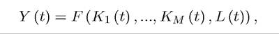
where Km denotes the mth type of capital and L is labor. F is homogeneous of degree 1 in all of its variables. Capital in each sector accumulates in the standard fashion, with
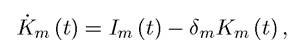
for m = 1,..., M. The resource constraint of the economy is
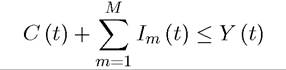
for all t.
(1) Write budget constraint of the representative household in this economy. Show that this can be done in two alternative and equivalent ways; first, with M separate assets, and second with only a single asset that is a claim to all of the capital in the economy.
(2) Define equilibrium and BGP allocations.
(3) Characterize the BGP by specifying the profit-maximizing decision of firms in each sector and the dynamic optimization problem of consumers.
(4) Write down the optimal growth problem in the form of a multidimensional currentvalue Hamiltonian and show that the optimum growth problem coincides with the equilibrium growth problem. Interpret this result.
(5) Characterize the transitional dynamics in this economy. Define and discuss the appropriate notion of saddle-path stability and show that the equilibrium is always saddle-path stable and the equilibrium dynamics can be reduced to those in the one-sector neoclassical growth model.
(6) Characterize the transitional dynamics under the additional assumption that investment is irreversible in each sector, i.e., Im (t) ≥ 0 for all t and each m = 1,...,M.
Exercise 8.37. Contrast the effects of taxing capital income at the rate τ in the Solow growth model and the neoclassical growth model. Show that capital income taxes have no 356
effect in the former, while they depress the effective capital-labor ratio in the latter. Explain why there is such a difference.