Exercises

EXERCISE 9.1. Prove that the allocation characterized in Proposition 9.1 is the unique com­petitive equilibrium. [Hint: first, show that there cannot be any equilibrium with pj > Pj_-ι for any j.

Exercise 9.2. Consider the following variant of economy with infinite number of commodi­ties and infinite number of individuals presented in Section 9.1. The utility of individual indexed i = j is

where β ∈ (0,1), and each individual has one unit of the good with the same index as his own.

(1) Define a competitive equilibrium for this economy.

(2) Characterize the set of competitive equilibria in this economy.

(3) Characterize the set of Pareto optima in this economy.

(4) Can all Pareto optima be decentralized without changing endowments? Can they be decentralized by changing endowments?

Exercise 9.3. Show that in the model of Section 9.2 the dynamics of capital stock are identical to those derived in the text even when δ < 1.

Exercise 9.4. In the baseline overlapping generations model, verify that savings s (w,R), given by (9.6), are increasing in the first argument, w. Provide conditions on the utility function u (∙) such that they are also increasing in their second argument (in the interest rate R).

Exercise 9.5. Prove Proposition 9.4

Exercise 9.6. Consider the canonical overlapping generations model with log preferences

for each household. Suppose that there is population growth at the rate n. Individuals work only when they are young, and supply one unit of labor inelastically.

(1) Define a competitive equilibrium and the steady-state equilibrium.

(2) Characterize the steady-state equilibrium and show that it is globally stable.

(3) What is the effect of an increase in g on the equilibrium?

(4) What is the effect of an increase in β on the equilibrium? Provide an intuition for this result.

Exercise 9.7. Consider the canonical model with log preferences, log (ci (t)) + β log (c2 (t)), and the general neoclassical technology F ( K, L) satisfying Assumptions 1 and 2. Show that multiple steady-state equilibria are possible in this economy.

Exercise 9.8. Consider again the canonical overlapping generations model with log prefer­ences and Cobb-Douglas production function.

(1) Define a competitive equilibrium.

(2) Characterize the competitive equilibrium and derive explicit conditions under which the steady-state equilibrium is dynamically inefficient.

(3) Using plausible numbers discuss whether dynamic inefficiency can arise in “realistic” economies.

(4) Show that when there is dynamic inefficiency, it is possible to construct an un­funded Social Security system which creates a Pareto improvement relative to the competitive allocation.

Exercise 9.9. Consider again the canonical overlapping generations model with log prefer­ences and Cobb-Douglas production function, but assume that individuals now work in both periods of their lives.

(1) Define a competitive equilibrium and the steady-state equilibrium.

(2) Characterize the steady-state equilibrium and the transitional dynamics in this econ­omy.

(3) Can this economy generate overaccumulation?

Exercise 9.10. Prove Proposition 9.7.

Exercise 9.11. Consider the overlapping generations model with fully funded Social Secu­rity. Prove that even when the restriction s (t) ≥ 0 for all t is imposed, no fully funded Social Security program can lead to a Pareto improvement.

Exercise 9.12. Consider an overlapping generations economy with the dynamically inef­ficient steady-state equilibrium. Show that the government can improve the allocation of resources by introducing national debt. [Hint: suppose that the government borrows from the current young and redistributes to the current old, paying back the current young the following period with another round of borrowing]. Contrast this result with the Ricardian equivalence result in Exercise 8.33 in Chapter 8.

Exercise 9.13. Prove Proposition 9.8.

Exercise 9.14. Consider the baseline overlapping generations model and suppose that the equilibrium is dynamically efficient, i.e., r* > n. Show that any unfunded Social Security system will increase the welfare of the current old generation and reduce the welfare of some future generation.

Exercise 9.15. Deriveeq. (9.31).

Exercise 9.16. Consider the overlapping generations model with warm glow preferences in Section 9.6, and suppose that preferences are given by

with η ∈ (0,1), instead of eq. (9.21). The production side is the same as in Section 9.6. Characterize the dynamic equilibrium of this economy.

Exercise 9.17. Consider the overlapping generations model with warm glow preferences in Section 9.6, and suppose that preferences are given by uι (ci (t)) + u.∙₂ (bi (t)), where uι and U2 are strictly increasing and concave functions. The production side is the same as in the text. Characterize a dynamic equilibrium of this economy.

Exercise 9.18. Characterize the aggregate equilibrium dynamics and the dynamics of wealth distribution in the overlapping generations model with warm glow preferences as in Section

9.6, when the per capita production function is given by the Cobb-Douglas form

Show that away from the steady state, there can be periods during which wealth inequality increases.

Exercise 9.19. * Generalize the results in Section 9.6 to an environment in which the pref­erences of an individual of generation t are given by

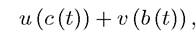
where c (t) denotes own consumption, b (t) is bequests, and u (∙) and v (∙) are strictly increas­ing, differentiable and strictly concave utility functions. Determine conditions on u (∙) and 390

v (∙) such that aggregate dynamics are globally stable. Provide conditions on u (∙) and v (∙) to ensure that asymptotically all individuals tend to the same wealth level.

EXERCISE 9.20. Show that the steady-state capital labor ratio in the overlapping generations model with impure altruism (of Section 9.6) can lead to overaccumulation, i.e., to k* > kg_θid. EXERCISE 9.21. Prove that given the perpetual youth assumption and population dynamics in eq. (9.34), at time t > 0, there will bes-year-olds for any

s ∈ {1, 2,...,t - 1}.

Exercise 9.22. * Consider the discrete-time perpetual youth model discussed in Section 9.7 and assume that preferences are logarithmic. Characterize the steady-state equilibrium and the equilibrium dynamics of the capital-labor ratio.

Exercise 9.23. Consider the continuous-time perpetual youth model of Section 9.8.

(1) Show that given L (0) = 1, the initial size of a cohort born at the time τ ≥ 0 is exp ((n — ν) τ).

(2) Show that the probability that an individual born at the time τ is alive at time t ≥ τ is exp (—ν (t — τ)).

(3) Derive eq. (9.40).

(4) Show that this equation would not apply at any finite time if the economy starts at t = 0 with an arbitrary age distribution.

Exercise 9.24. Derive eq. (9.46). [Hint: first integrate the flow budget constraint of the individual, (9.41) using the transversality condition (9.45) and then use the Euler equation (9.44)].

EXERCISE 9.25. Generalize the analysis of the continuous-time perpetual youth model of Section 9.8 to an economy with labor-augmenting technological progress at the rate g. Prove that the steady-state equilibrium is unique and globally (saddle-path) stable. What is the impact of a higher rate of technological progress?

Exercise 9.26. Linearize the differential equations (9.43) and (9.49) around the steady state, (k*,c*), and show that the linearized system has one negative and one positive eigenvalue.

Exercise 9.27. Determine the effects of n and ν on the steady-state equilibrium (k*,c*) in the continuous-time perpetual youth model of Section 9.8.

Exercise 9.28. (1) Derive eq.’s (9.52) and (9.53).

(2) Show that for ζ sufficiently large, the steady-state equilibrium capital-labor ratio, k*, can exceed k_gold, so that there is overaccumulation. Provide an intuition for this result.

Exercise 9.29. Consider the continuous-time perpetual youth model with a constant flow of government spending G. Suppose that this does not affect consumer utility and that lump­sum taxesare allowed. Specify the government budget constraint as in Exercise

8.33 in Chapter 8. Prove that contrary to the Ricardian Equivalence result in Exercise 8.33, the sequence of taxes affects the equilibrium path of capital-labor ratio and consumption. Interpret this result and explain the difference between the overlapping generations model and the neoclassical growth model.

Exercise 9.30. * Consider the continuous-time perpetual youth model with labor income All markets are competitive, the labor supply is normalized to 1, capital fully depreciates after use, and the government imposes a linear tax on capital income at the rate τ and uses the proceeds for government consumption. Consider two specifications of preferences:

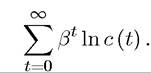
• All agents are infinitely lived, with preferences

• An overlapping generations model where agents work in the first period, and con­sume the capital income from their savings in the second period. The preferences of a generation born at time t, defined over consumption when young and old, are given by

(1) Characterize the equilibria in these two economies, and show that in the first econ­omy, taxation reduces output, while in the second, it does not.

(2) Interpret this result, and in the light of this result discuss the applicability of models that try to explain income differences across countries with differences in the rates of capital income taxation.