Exercises

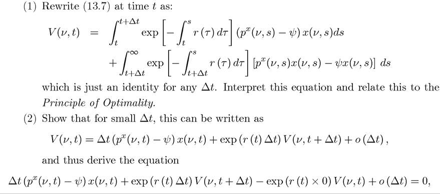
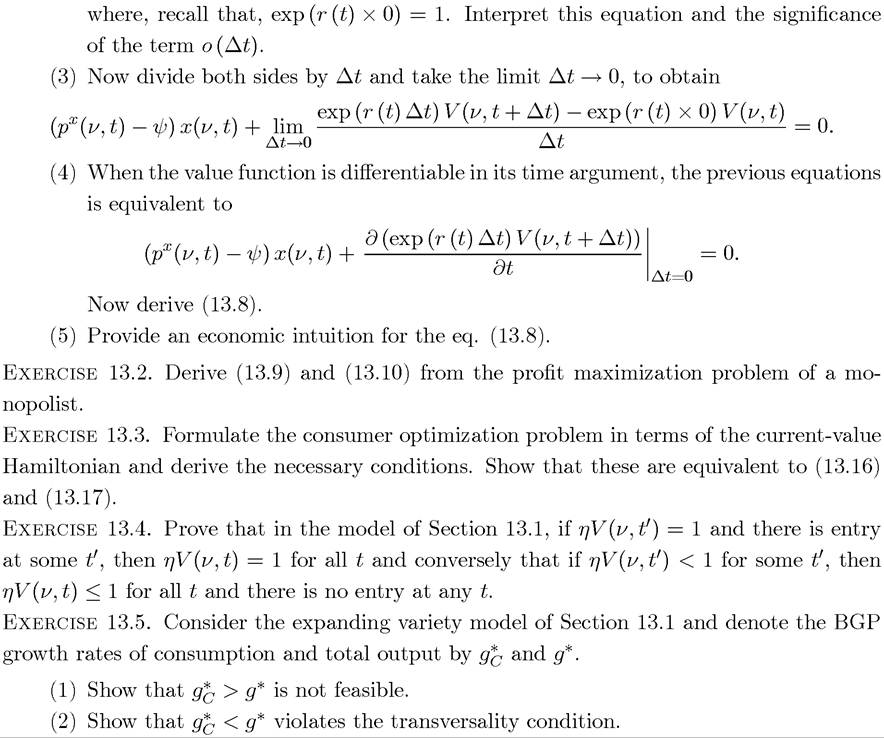
Exercise 13.1. This exercise asks you to derive (13.8) from (13.7).

Exercise 13.6.

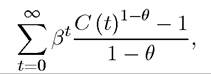
with β ∈ (0,1) and θ ≥ 0. Production technology is the same as in the text and the innovation possibilities frontier of the economy is given by

N (t +1) - N (t) = ηZ (t).

(1) Define the equilibrium in BGP allocations.

(2) Characterize the BGP and compare the structure of the equilibrium to that in Section 13.1.

(3) Show that there are no transitional dynamics, so that starting with any N (0) > 0, the economy grows at a constant rate.

Exercise 13.7. Complete the proof of Proposition 13.1, in particular, showing that condition

(13.21) is sufficient for the transversality condition to be satisfied.

Exercise 13.8. Consider a world economy consisting of j = 1,...,M economies. Suppose that each of those are closed and have access to the same production and R&D technology as described in Section 13.1. The only differences across countries are in the size of labor force, Lj, productivity of R&D, ηj, and discount rate ρj. Also assume that one unit of R&D expenditure costs ζj units of final good in country j, and this varies across countries. There are no technological exchanges across countries.

(1) Define the “world equilibrium” in which each country is in equilibrium in analogy with the equilibrium path of the one country economy in Section 13.1.

(2) Characterize the world equilibrium. Show that in the world equilibrium, each coun­try will grow at a constant rate starting at t = 0. Provide explicit solutionse for these growth rates.

(3) Show that except in “knife-edge” cases, output in each country will grow at a dif­ferent long-run rate.

(4) Now return to the discussion in Chapters 3 and 8 regarding the effect of policy and taxes on long-run income per capita differences. Show that, in the model discussed in this exercise, arbitrarily small differences in policy or discount factors across countries will lead to “infinitely large” differences in long-run income per capita. Does this resolve the empirical challenges discussed in those chapters? Does the environment in this exercise provide a satisfactory model for the study of long-run income per capita differences across countries? If yes, please elaborate how such a model can be mapped to reality. If not, explain which features of the model appear unsatisfactory to you and how you would want to change them.

Exercise 13.9. (1) Verify that Theorem 7.14 from Chapter 7 can be applied to the

social planner’s problem in Section 13.1.

(2) Derive the consumption growth rate in the socially-planned economy, (13.22). Exercise 13.10. Consider the expanding input variety model of Section 13.1. Show that it is possible for the equilibrium allocation to satisfy the transversality condition, while the social planner’s solution may violate it. Interpret this result. Does it imply that the social planner’s allocation is less compelling?

Exercise 13.11. Complete the proof of Proposition 13.3, in particular showing that the Pareto optimal allocation always involves a constant growth rate and no transitional dynam­ics.

Exercise 13.12. Consider the expanding input variety model of Section 13.1.

(1) Suppose that a benevolent government has access only to research subsidies, which can be financed by lump-sum taxes. Can these subsidies be chosen so as to ensure that the equilibrium growth rate is the same as the Pareto optimal growth rate? Can they be used to replicate the Pareto optimal equilibrium path? Would it be desirable for the government to use subsidies so as to achieve the Pareto optimal growth rate (from the viewpoint of maximizing social welfare at time t = 0)?

(2) Suppose that the government now has only access to subsidies to machines, which can again be financed by lump-sum taxes.

(3) Will the combination of subsidies to machines and subsidies to research be better than either of these two policies by themselves?

EXERCISE 13.13. Consider the expanding input variety model of Section 13.1 and assume that corporate profits are taxed at the rate τ.

(1) Characterize the equilibrium allocation.

(2) Consider two economies with identical technologies and identical initial conditions, but with different corporate tax rates, τ and τ⁰. Determine the relative income of these two economies (possibly as a function of time).

Exercise 13.14. * Consider the expanding input variety model of Section 13.1, with one difference. A firm that invents a new machine receives a patent, which expires at the Poisson rate ι. Once the patent expires, that machine is produced competitively and is supplied to final good producers at marginal cost.

(1) Characterize the equilibrium in this case and show how the equilibrium growth rate depends on ι. [Hint: notice that there will be two different types of machines, supplied at different prices].

(2) What is the value of ι that maximizes the equilibrium rate of economic growth?

(3) Show that a policy ofdoes not necessarily maximize social welfare at time t = 0.

Exercise 13.15. Consider the formulation of competition policy in subsection 13.1.6.

(1) Characterize the equilibrium fully.

(2) Write down the welfare of the representative household at time t = 0 in this equi­librium.

(3) Maximize this welfare function by choosing a value of γ.

(4) Why is the optimal value of γ not equal to someProvide an

interpretation in terms of the tradeoff between level and growth effects.

(5) What is the relationship between the optimal value ofInterpret.

Exercise 13.16. Complete the proof of Proposition 13.4. In particular, show that the equi­librium path involves no transitional dynamics and that under (13.31), the transversality condition is satisfied.

EXERCISE 13.17. Characterize the Pareto optimal allocation in the economy of Section 13.2. Show that it involves a constant growth rate greater than the equilibrium growth rate in Proposition 13.4 and no transitional dynamics.

Exercise 13.18. Derive eq. (13.35) and explain why the denominator is equal to r* — n. Exercise 13.19. Consider the model of endogenous technological progress with limited knowledge spillover as discussed in Section 13.3.

(1) Characterize the transitional dynamics of the economy starting from an arbitrary N (0) > 0.

(2) Characterize the Pareto optimal allocation and compare it to the equilibrium allo­cation in Proposition 13.5.

(3) Analyze the effect of the following two policies: first, a subsidy to research; second, a patent policy, where each patent expires at the rate ι > 0. Explain why the effects of these policies on economic growth are different than their effects in the baseline endogenous growth model.

EXERCISE 13.20. Consider the model in Section 13.3. Suppose that there are two economies with identical preferences, technology and initial conditions, except country 1 starts with population Li (0) and country 2 starts with L₂ (0) > Lι (0). Show that income per capita is always higher in country 2 than in country 1.

Exercise 13.21. Consider the lab-equipment model of Section 13.1, but modify the innova­tion possibilities frontier to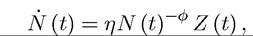

where φ > 0.

(1) Define an equilibrium.

(2) Characterize the market clearing factor prices and determine the free-entry condi­tion.

(3) Show that without population growth, there will be no sustained growth in this economy.

(4) Now consider population growth at the exponential rate n, and show that this model generates sustained equilibrium growth as in the model analyzed in Section 13.3.

EXERCISE 13.22. Consider the baseline endogenous technological change model with expand­ing machine varieties in Section 13.1. Suppose that x’s now denote machines that do not immediately depreciate. In contrast, once produced these machines depreciate as an expo­nential rate δ. Preferences and the rest of the production structure remain unchanged.

(1) Define the equilibrium in BGP allocations.

(2) Formulate the maximization problem of producers of machines. [Hint: it is easier to formulate the problem in terms of machine rentals rather than machine sales].

(3) Characterize the equilibrium in this economy and show that all the results are iden­tical to those in Section 13.1.

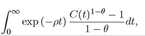
Exercise 13.23. Consider the following model. Population at time t is L (t) and grows at the constant rate n (i.e.,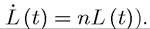All agents have preferences given by

where C is consumption defined over the final good of the economy. This good is produced as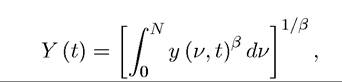

where y (ν, t) is the amount of intermediate good ν used in production at time t. The production function of each intermediate is

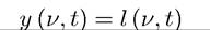
where l (ν, t) is labor allocated to this good at time t.

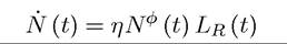
New goods are produced by allocating workers to the R&D process, with the production function

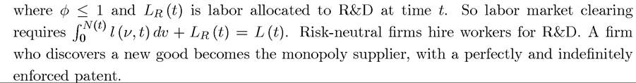
(1) Characterize the BGP in the case where φ = 1 and n = 0, and show that there are no transitional dynamics.

(2) Now suppose that φ = 1 and n > 0. What happens? Interpret.

(3) Now characterize the BGP when φ < 1 and n > 0. Does the growth rate depend on L? Does it depend on n? Why? Do you think that the configuration φ < 1 and n > 0 is more plausible than the one with φ = 1 and n = 0?

Exercise 13.24. Derive eq. (13.43). [Hint: use the first-order condition between two prod­ucts ν and V, and then substitute into the budget constraint of the representative household with total expenditure denoted by C (t)].

Exercise 13.25. Using (13.43) and the choice of numeraire in (13.44), set up the consumer optimization problem in the form of the current-value Hamiltonian (derive the consumer’s budget constraint explicitly). Derive the consumer Euler equation (13.45).

Exercise 13.26. Consider the model analyzed in Section 13.4.

(1) Show that the allocation described in Proposition 13.6 always satisfies the transver- sality condition.

(2) Show that in this model there are no transitional dynamics.

(3) Characterize the Pareto optimal allocation and show that the equilibrium growth rate in Proposition 13.6 is less than the growth rate in the Pareto optimal allocation.