Exercises

EXERCISE 14.1. Prove that in the baseline model of Schumpeterian growth in Section 14.1, BGP R&D towards different types of machines must be equal to some z*. [Hint: use (14.13) together with (14.12)].

Exercise 14.2. (1) Prove that in the baseline model of Schumpeterian growth in Sec­

tion 14.1, all R&D will be undertaken by entrants, and there will never be R&D by incumbents. [Hint: rewrite (14.12) by allowing for a choice of R&D investments].

(2) Now suppose that the flow rate of success of R&D is φη∕q for an incumbent as opposed to η∕q for an entrant. Show that for any value of φ ≤ 1/ (λ — 1), the incumbent will still choose zero R&D. Explain this result.

Exercise 14.3. The baseline endogenous technological change models, including the model of Schumpeterian growth in this chapter, assume that new products are protected by perpetual patents. This exercise asks you to show that this is not strictly necessary in the logic of these models. Suppose that there is no patent protection for any innovation, but copying an innovator requires a fixed cost ε > 0. Any firm, after paying this cost, has access to the same technology as the innovator. Prove that in this environment there will be no copying and all the results of the model with fully-enforced perpetual patents apply.

Exercise 14.4. Complete the proof of Proposition 14.1. In particular, verify that the equi­librium growth rate is unique, strictly positive and such that the transversality condition

(14.15) is satisfied.

Exercise 14.5. Prove Proposition 14.2.

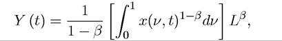
Exercise 14.6. Modify the baseline model of Section 14.1 so that the aggregate production function for the final good is

All the other features of the model remain unchanged.

(1) Show that with this production function, a BGP does not exist. Explain why this is.

(2) What would you change in the model to ensure the existence of a BGP.

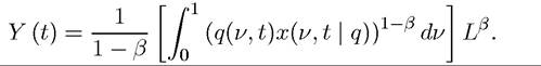
Exercise 14.7. * In the baseline Schumpeterian growth model, instead of (14.3), suppose that the production function of the final good sector is given by

Suppose also that producing one unit of an intermediate could of quality q costs ψq^² and that one unit of final good devoted to research on the machine line with quality q generates a flow rate of innovation equal toCharacterize the equilibrium of this economy and determine what combinations of the parameterswill ensure balanced growth.

Exercise 14.8. (1) Verify that Theorem 7.14 from Chapter 7 can be applied to the

social planner’s problem in the baseline Schumpeterian model of Section 14.1.

(2) Derive eq. (14.24).

Exercise 14.9. Show that condition (14.5) is sufficient to ensure that a firm that innovates will set the unconstrained monopoly price. [Hint: first suppose that the innovator sets the monopoly price ψq∕ (1 — β) for a product of quality q. Then, consider the firm with the next highest quality, λ^-1q. Suppose that this firm sells at marginal cost, ψλ^-1q. Then, find the value of λ such that final good producers are indifferent between buying a machine of quality q at the price ψq∕ (1 — β} versus a machine of quality λ^-1q at the price ψλ^-1q.]

Exercise 14.10. Analyze the baseline model of Schumpeterian growth in Section 14.1 as­suming that (14.5) is not satisfied.

(1) Show that monopolists will set a limit price.

(2) Characterize the BGP equilibrium growth rate.

(3) Characterize the Pareto optimal allocation and compare it to the equilibrium al­location. How does the comparison differ from the case in which innovations were drastic?

(4) Now consider a hypothetical economy in which the previous highest-quality producer disappears so that the monopolist can charge a markup of 1/ (1 — β) instead of the limit price. Show that the BGP growth rate in this hypothetical economy is strictly greater than the growth rate characterized in 2 above. Explain this result.

Exercise 14.11. Suppose that there is constant exponential population growth at the rate n. Modify the baseline model of Section 14.1 so that there is no scale effect and the economy grows at the constant rate (with positive growth of income per capita). [Hint: suppose that one unit of final good spent on R&D for improving the machine of quality q leads to flow rate of innovation equal to η∕q^φ, where φ > 1].

Exercise 14.12. * Consider a version of the model of Schumpeterian growth in which the x’s do not depreciate fully after use (similar to Exercise 13.22 in the previous chapter). Preferences and the rest of the production structure are the same as in the baseline model in Section 14.1.

(1) Define the equilibrium in BGP allocations.

(2) Formulate the maximization problem of a monopolist with the highest quality ma­chine.

(3) Show that, contrary to Exercise 13.22, the results are different than those in Section 14.1. Explain why depreciation of machines was not important in the expanding varieties model, but it is important in Schumpeterian models.

Exercise 14.13. Consider a version of the model of Schumpeterian growth in which inno­vations reduce costs instead of increasing quality. In particular, suppose that the aggregate

production function is given by

and the marginal cost of producing machine variety ν at time t is given by MC (ν, t).

(1) Define the equilibrium and BGP allocations.

(2) Specify a form of the innovation possibilities frontier that is consistent with balanced growth.

(3) Derive the BGP growth rate of the economy and show that there are no transitional dynamics.

(4) Compare the BGP growth rate to the Pareto optimal growth rate of the economy. Can there be excessive innovations?

(5) What are the similarities and differences between this model and the baseline model presented in Section 14.1.

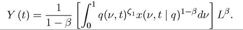
Exercise 14.14. Consider the model in Section 14.2, with R&D performed by workers.

Suppose instead that the aggregate production function for the final good is given by

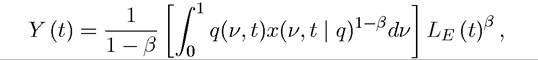
where Le (t) denotes the number of workers employed in final good production at time t.

(1) Show that in this case, there will only be R&D for the machine with the highest q(ν,t).

(2) How would you modify the model so that the equilibrium has balanced R&D across sectors?

EXERCISE 14.15. Consider the model of Schumpeterian growth in Section 14.1, with one dif­ference: conditional on success an innovation generates a random improvement of λ over the previous technology, where the distribution function of λ is H (λ) and has support

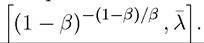
(1) Define the equilibrium and BGP allocations.

(2) Characterize the BGP and specify restrictions on parameters so that the transver- sality condition is satisfied.

(3) Why did we assume that the lower support ofHow would the analysis

change if this were relaxed?

(4) Show that there are no transitional dynamics in this economy.

(5) Compare the BGP growth rate to the Pareto optimal growth rate of the economy.

Exercise 14.16. In the model of Section 14.2 show that the economy experiences no growth of output for intervals of average length 1∕ηLR.

Exercise 14.17. (1) Prove Proposition 14.4, in particular verifying that the allocation

described there is unique, that the average growth rate is given by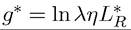and

that condition (14.27) is necessary and sufficient for the existence of the equilibrium described in the proposition.

(2) Explain why the growth rate features ln λ rather than λ — 1 as in the model of Section 14.1.

Exercise 14.18. Consider the one-sector Schumpeterian model in discrete time. Suppose as in the model in Section 14.2 that consumers are risk neutral, there is no population growth, and the final good sector has the production function given by (14.25). There is a linear production technology for intermediate goods whereby any type of intermediate good (that has been invented) can be produced at the marginal cost of ψ units of the final good. Assume also that the R&D technology is such that Lr > 0 workers employed in research at time t will necessarily lead to an innovation for time t + 1, and the number of workers used in research simply determines the quality of the innovation via the function Λ (Lr), that is, if date t quality is q, the new, date t + 1 machine will have qualityAssume that

there will be innovation only if Lr > 0 and Λ (∙) is strictly increasing, differentiable, strictly concave and satisfies the appropriate Inada conditions.

(1) Define equilibrium and BGP allocations.

(2) Characterize the BGP and specify restrictions on parameters so that the transver- sality condition is satisfied. [Hint: to simplify the algebra, you may wish to assume that once the new machine is invented, the old one cannot be used any longer, so that there is no limit pricing].

(3) Compare the BGP growth rate to the Pareto optimal growth rate of the economy. Show that the size of innovations is always too small relative to the size of innovations in the Pareto optimal allocation.

Exercise 14.19. * Consider the one-sector Schumpeterian model in discrete time analyzed in the previous exercise, except that now Λ (∙) denotes the probability of innovation and each innovation improves the quality of a machine q to λq, where λ > 1. Suppose that when a new innovation arrives a fraction φ of workers employed in the final good production will not be able to adapt to this new technology and will need to remain unemployed for one time period to “retool”.

(1) Define the equilibrium and BGP allocations. [Hint: also specify the number of unemployed workers in equilibrium].

(2) Defined the appropriate generalization of the BGP for this economy and determine the number of unemployed workers in this equilibrium.

(3) Show that the economy will experience bursts of unemployment, followed by periods of full employment.

(4) Show that a decline in ρ will increase the average growth rate and the average unemployment rate in the economy.

Exercise 14.20. * Derive eq.’s (14.28)-(14.29).

Exercise 14.21. * Consider the model discussed in subsection 14.2.2.

(1) Choose a functional form for η (∙) such that eq.’s (14.29) have solutionsand

Explain why, when such solutions exist, there is a perfect foresight equilibrium with two-period endogenous cycles.

(2) Show that even when solutions exist, there also exists a steady-state equilibrium with constant research.

(3) Show that when such solutions do not exist, there exists an equilibrium which ex­hibits oscillatory transitional dynamics converging to the steady state characterized in 2 above.

Exercise 14.22. * Show that the qualitative results of the model in subsection 14.2.2 gen­eralize when there is a single firm undertaking research, thus internalizing the effect of Lr on η (Lr).

Exercise 14.23. Suppose that in the model of Section 14.3 incumbents also have access to the radical innovation technology used by entrants. Show that there cannot existing equilibrium in which incumbents undertake positive R&D with this technology. [Hint: use the free-entry condition for entrants together with to condition that makes such investments profitable for incumbents and derive a contradiction].

Exercise 14.24. Set up the social planner’s problem (of maximizing the utility of the rep­resentative household) in Section 14.3.

(1) Show that this maximization problem corresponds to a concave current-value Hamil­tonian and derive the unique solution to this problem. Show that this solution in­volves the consumption of the representative household growing at a constant rate at all points.

(2) Show that the social planner will tend to increase growth because she avoids the monopoly markup over machines.

(3) Show that the social planner will tend to choose lower entry because of the negative externality in the research process.

(4) Give numerical examples in which the growth rate in the Pareto optimal allocation is greater than or less than the decentralized growth rate.

Exercise 14.25. Consider the model of Section 14.3 and suppose that the R&D technology of the incumbents for innovation is such that if an incumbent with a machine of quality q spends an amount zq for incremental innovations, then the flow rate of innovation is φ (z) (and this innovation again increases the quality of the incumbent’s machine to λq). Assume that φ (z) is strictly increasing, strictly concave, differentiable, and satisfies and

(1) Focus on steady-state equilibria and conjecture that V (q) = vq. Using this con­jecture, show that incumbents will choose R&D intensity z* such that (λ — 1) v = φ' (z*). Combining this equation with the free-entry condition for entrants and the equation for growth rate given by (14.54), show that there exists a unique BGP equilibrium (under the conjecture that V (q) is linear).

(2) Is it possible for an equilibrium to involve different levels of z for incumbents with different quality machines?

(3) In light of your answer to 2, what happens if we consider the “limiting case” of this model where φ (z) = constant?

(4) Show that this equilibrium involves positive R&D both by incumbents and entrants.

(5) Now introduce taxes on R&D by incumbents and entrants at the rates Ti and τ_e.

Show that, in contrast to the results in Proposition 14.7, the effects of both taxes on growth are ambiguous. What happens if η (z) = constant?

Exercise 14.33. * Modify the model presented in Section 14.4 such that followers can now use the innovation of the technological leader and immediately leapfrog the leader, but in this case they have to pay a license fee of ζ to the leader.

(1) Characterize the BGP in this case

(2) Write the value functions.

(3) Explain why licensing can increase the growth rate of the economy in this case, and contrast this result with the one in Exercise 12.9, where licensing was never used in equilibrium. What is the source of the difference between the two sets of results?

Exercise 14.34. (1) What is the effect of competition on the rate of growth of the

economy in a standard product variety model of endogenous growth? What about the quality-ladder model? Explain the intuition.

(2) Now consider the following one-period model. There are two Bertrand duopolists, producing a homogeneous good. At the beginning of each period, duopolist 1's mar­ginal cost of production is determined as a draw from the uniform distribution and the marginal cost of the second duopolist is determined as an independent draw fromBoth cost realizations are observed and then prices are set. Demand is given by Q = A — P, with A > 2max

(a) Characterize the equilibrium pricing strategies and calculate expected ex ante profits of the two duopolists.

(b) Now imagine that both duopolists start with a cost distributiorand can

undertake R&D at cost μ. If they do, with probability η, their cost distribution shifts towhereFind the conditions under which one of the

duopolists will invest in R&D and the conditions under which both will.

(c) What happens when c declines? Interpreting the decline in c as increased com­petition, discuss the effect of increased competition on innovation incentives. Why is the answer different from that implied by the baseline endogenous tech­nological change models of expanding varieties or Schumpeterian growth?