Growth with Externalities
The model that started much of endogenous growth theory and revived economists’ interest in economic growth was Paul Romer’s (1986) paper. Romer’s objective was to model the process of “knowledge accumulation”.
He realized that this would be difficult in the context of a competitive economy. His initial solution (later updated and improved in his and others’ work during the 1990s) was to consider knowledge accumulation to be a byproduct of capital accumulation. In other words, Romer introduced technological spillovers, similar to those discussed in the context of human capital in Chapter 10. While arguably crude, this captures an important dimension of knowledge, that knowledge is a largely non-rival good—once a particular technology has been discovered, many firms can make use of this technology without preventing others using the same knowledge. Non-rivalry does not imply knowledge is also non-excludable (which would have made it a pure public good). A firm that discovers a new technology may use patents or trade secrecy to prevent others from using it, for example, in order to gain a competitive advantage. These issues will be discussed in the next part of the book. For now, it suffices to note that some of the important characteristics of “knowledge” and its role in the production process can be captured in a reduced-form way by introducing technological spillovers. I next discuss a version of the model in Romer’s (1986) paper, which introduces such technological spillovers as the engine of economic growth. While the type of technological spillovers used in this model are unlikely to be important in practice, this model is a good starting point for our analysis of endogenous technological progress, since its similarity to the baseline AK economy makes it a very tractable model of knowledge accumulation.11.4.1. Preferences and Technology.
Consider an economy without any population growth (we will see why this is important) and a production function with labor-augmenting knowledge (technology) that satisfies the standard assumptions, Assumptions 1 and 2. For reasons that will become clear, instead of working with the aggregate production function, let us assume that the production side of the economy consists of a set [0,1] of firms. The production function facing each firm i ∈ [0,1] is (11.35) Yi (t) = F (Ki (t),A (t) Li (t)), where Ki (t) and Li (t) are capital and labor rented by a firm i. Notice that A (t) is not indexed by i, since it is technology common to all firms. Let us normalize the measure of final good producers to 1, so that the following market clearing conditions apply: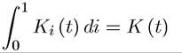
and
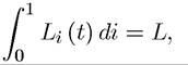
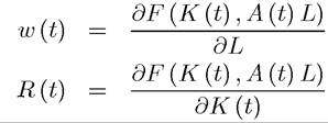
where L is the constant level of labor (supplied inelastically) in this economy. Firms are competitive in all markets, which implies that they will all hire the same capital to effective labor ratio, and moreover, factor prices will be given by their marginal products, thus
The key assumption of Romer (1986a) is that although firms take A (t) as given, this stock of technology (knowledge) advances endogenously for the economy as a whole. In particular, Romer assumes that this takes place because of spillovers across firms, and attributes spillovers to physical capital. Lucas (1988) develops a similar model in which the structure is identical, but spillovers work through human capital (while Romer has physical capital externalities, Lucas has human capital externalities).
The idea of externalities is not uncommon to economists, but both Romer and Lucas make an extreme assumption of sufficiently strong externalities such that A (t) can grow continuously at the economy level.
In particular, Romer assumes
so that the knowledge stock of the economy is proportional to the capital stock of the economy. This can be motivated by “learning-by-doing” whereby, greater investments in certain sectors increases the experience (of firms, workers, managers) in the production process, making the production process itself more productive. Alternatively, the knowledge stock of the economy could be a function of the cumulative output that the economy has produced up to now, thus giving it more of a flavor of “learning-by-doing”. Note also that (11.35) and (11.36) imply that the aggregate production function of this economy exhibits increasing returns to scale. As discussed in detail in the next part of the book, this is a very common feature of models of endogenous growth.
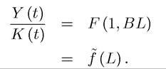
In any case, substituting for (11.36) into (11.35) and using the fact that all firms are functioning at the same capital-effective labor ratio, the production function of the representative firm is
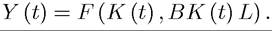
Using the fact that F (∙, ∙) is homogeneous of degree 1,
Output per capita can therefore be written as:
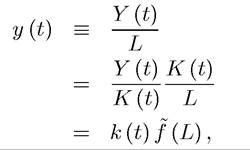
where again k (t) ? K (t) /L is the capital-labor ratio in the economy.
As in the standard growth model, marginal products and factor prices can be expressed in terms of the normalized production function, now f (L). In particular,  and
and

which is constant.
11.4.2. Equilibrium.
A competitive equilibrium is defined similarly to the neoclassical growth model, as a path of consumption and capital stock for the economy, that maximize the utility of the representative household and wage and rental rates
  that clear markets. The important feature is that because the knowledge spillovers, as specified in (11.36), are external to each firm, factor prices are given by (11.37) and (11.38)—that is, they do not price the role of the capital stock in increasing future productivity.
 Since the market rate of return is r (t) = R (t) — δ, it is also constant. The usual consumer Euler equation (e.g., (11.4) above) then implies that consumption must grow at the constant rate,

It is also clear that capital grows exactly at the same rate as consumption, so the rate of capital, output and consumption growth are all given by gβ as given by (11.39)—see Exercise 11.16.
Let us assume that

so that there is positive growth, but also that growth is not fast enough to violate the transversality condition, in particular, 
PROPOSITION 11.5. Consider the above-described Romer model with physical capital externalities. Suppose that conditions (11.40) and (11.41) are satisfied. Then, there exists a unique equilibrium path where starting with any level of capital stock K (0) > 0, capital, output and consumption grow at the constant rate (11.39).
Proof. Much of this proposition is proved in the preceding discussion. You are asked to verify the transversality conditions and show that there are no transitional dynamics in Exercise 11.17.
?This proposition (and the accompanying analysis) therefore provides us with the first example of endogenous technological change. The technology of the economy, A (t) as given in (11.36), evolves endogenously as a result of the investment decisions of firms. Consequently, the growth rate of the economy is endogenous, even though none of the firms purposefully invest in research or in acquiring new technologies.
Population must be constant in this model because of the scale effect. Since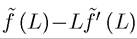 is always increasing in L (by Assumption 1), a higher population (labor force) L leads to a higher growth rate. The scale effect refers to this relationship between population and the equilibrium rate of economic growth. Now if population is growing, the economy will not admit a steady state and the growth rate of the economy will increase over time (output reaching infinity in finite time and violating the transversality condition). The implications of positive population growth are discussed further in Exercise 11.18. Scale effects and how they can be removed will be discussed in detail in Chapter 13.
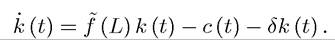
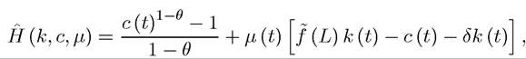
11.4.3. Pareto Optimal Allocations. Given the presence of externalities, it is not surprising that the decentralized equilibrium characterized in Proposition 11.5 is not Pareto optimal. To characterize the allocation that maximizes the utility of the representative household, let us again set up the current-value Hamiltonian and look for a candidate path that satisfies the conditions in Theorem 7.13 (see Exercise 11.15). The per capita accumulation equation for this economy can be written as
The current-value Hamiltonian is
and has the necessary conditions:
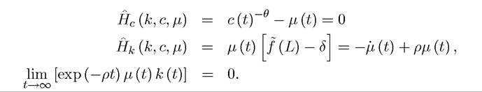
Using standard arguments (recall Section 7.7 in Chapter 7), it is straightforward to verify that the current-value Hamiltonian satisfies the conditions in Theorem 7.14, so that these conditions are sufficient for a Pareto optimum (see again Exercise 11.15).
Combining these equations immediately yields that the social planner’s allocation will also have a constant growth rate for consumption (and output) given by
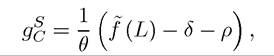
which is always greater than as given by (11.39)—since
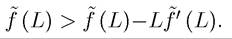 Essentially,
the social planner takes into account that by accumulating more capital, she is improving productivity in the future.
Since this effect is external to the firms, the decentralized economy fails to internalize this spillover. Therefore:PROPOSITION 11.6. In the above-described Romer model with physical capital externalities, the decentralized equilibrium is Pareto suboptimal and grows at a slower rate than the allocation that would maximize the utility of the representative household.
Exercise 11.19 asks you to characterize various different types of policies that can close the gap between the equilibrium and Pareto optimal allocations.
11.5.