Indeterminacy, Self-Fulfilling Prophecies, and Sunspots
The models we have analyzed in section 22.3 are linear models. Indeed, most of the models we have analyzed formally throughout this text are treated as local linear approximations of nonlinear models around a unique steady state.
However, even if a nonlinear model satisfies the saddle point property locally, it may have more than one nonexplosive solution, which implies global indeterminacy. As a result, which solution will apply may depend on extraneous beliefs.Consider the following model, which is a nonlinear version of the model in (22.1). For simplicity, let us ignore exogenous variables.9

where yt ∈ [0, 1] and |a| < 1. This model has two solutions. One obvious solution is

A second solution is that
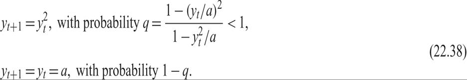
Therefore, the model has at least two nonexplosive solutions. In the first, the endogenous variable y is equal to the constant a at all times. In the second solution it follows stochastic cycles, although there is no intrinsic uncertainty.
As suggested by Azariadis [1981], which solution will prevail can be a self-fulfilling prophecy. If economic agents believe in the constant solution, the economy will settle at a. If they believe in the equilibrium with stochastic cycles, the economy will display stochastic cycles.
More generally, as demonstrated by Cass and Shell [1983], in economies with even small departures from the Arrow-Debreu assumptions of full markets, equilibria may display the property that agent’s allocations are different across states of nature, even though nothing fundamental is different across these states of nature.
Cass and Shell [1983] refer to equilibria with such a property as equilibria where sunspots matter. They define sunspots as random variables that have no direct influence on economic fundamentals, such as preferences, endowments, or technologies.10The sunspot theorem of Cass and Shell [1983] has profound implications for DSGE models, because it permits the possibility that sunspots (or “animal spirits,” in the terminology of Keynes [1936]) are quite consistent with the existence of a rational expectations equilibrium.
Given that many of the models we have analyzed are essentially nonlinear dynamic models characterized by departures from the Arrow-Debreu assumption of full markets, one cannot exclude multiple equilibria, self-fulfilling prophecies, and sunspots as easily as unstable bubbles. The Calvo [1988] debt model analyzed in chapter 21 is an example of such a model, in which there are multiple equilibria, and self-fulfilling prophecies play a major role in which equilibrium prevails. Other widely used examples of models with multiple equilibria and incomplete markets that we shall consider below are nonlinear OLG models with money, such as the Samuelson [1958] monetary model. In OLG models, there are no markets for the welfare or future generations, and hence the Arrow-Debreu assumption of full markets is not satisfied.
22.4.1 The Samuelson OLG Model with Money, Revisited
Consider a more general version of the Samuelson [1958] OLG model with money than the one first introduced in chapter 12.
The household born in period t lives for two periods and has a perishable endowment equal to Y1 in its first period of life and to Y2 in its second period of life. The only nonperishable asset is money M, held by old households, who were born in period t − 1, and who are in the second (and last) period of life.
The young households maximize the intertemporal utility function
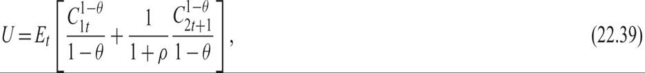
subject to the intertemporal budget constraint

where C1 is the level of consumption of the young; C2 is the level of consumption of the old; Pt is the price of consumer goods in period t; and EtPt+1 is the rational expectation of the price of consumer goods in period t + 1, conditional on the information set available in period t.
In addition, ρ > 0 is the pure rate of time preference, and 1/θ > 0 is the elasticity of intertemporal substitution.11First-period savings can only be held in the form of money, which yields no interest. Hence, money demand by the young is given by

Note that from the intertemporal budget constraint, the gross return on savings and money holdings Rt is equal to

where π is the inflation rate. Therefore, the gross return on savings and money is inversely related to expected inflation.
The savings of the young are equal to the dissavings of the old, who exchange their money holdings for consumer goods. Hence, the money supply by the old is equal to

Equilibrium in the money market implies

where M is the exogenously given money stock. Equilibrium in the money market also implies equilibrium in the goods market, in the sense that aggregate current income, Y = Y 1 + Y 2, is consumed by either the young or the old.
The Lagrange function for the problem of the young is given by
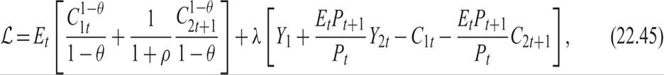
where λ is the Lagrange multiplier measuring the marginal utility of wealth.
From the first-order conditions for a maximum, we have
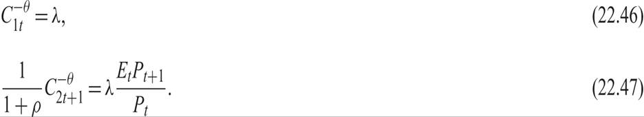
Eliminating λ between the two first-order conditions, after some rearrangement, we get the Euler equation for consumption:
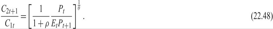
Figure 22.3 presents the combinations of C1t and C2t+1 that satisfy the Euler equation for consumption and the household intertemporal budget constraint as the gross return on money Rt = Pt/Pt+1 rises. These points trace out the offer curve of young households, which is defined by the points of tangency of the intertemporal budget constraint for different rates of gross return of money (savings) with the highest possible indifference curve.12
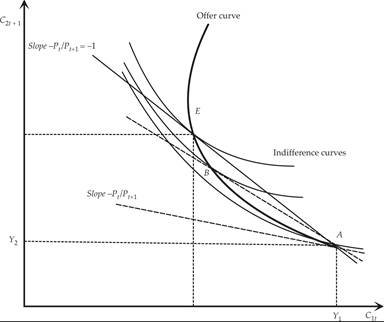
Figure 22.3 Equilibrium consumption in the Samuelson OLG model.
At point A, the gross return of money is sufficiently low, so that the household consumes its current endowment in both periods, and there are no savings and no demand for money. At point B, the gross return of money is sufficiently high to induce the household to save part of its income in its first period of life and thus to hold positive real money balances. At point E, the gross rate of return of money is equal to one, and prices and real money balances are constant.
If the elasticity of intertemporal substitution of consumption is higher than unity, then the offer curve is negatively sloped throughout. If it is lower than unity and the income effect dominates, after some point, the offer curve turns positively sloped, as an increase in the gross return on money causes savings and money demand to decline.
Eliminating C2t between the intertemporal budget constraint and the Euler equation for consumption, we find that the savings of the young is determined by
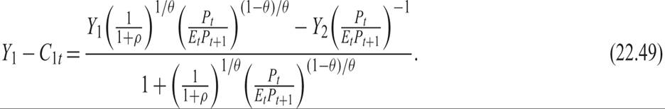
Because the savings of the young is equal to money demand, it follows that
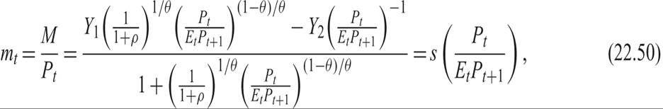
where m denotes real money balances, and s denotes the savings and money demand function, which depends on the expected gross return on real money balances.13
It is straightforward to prove that only if the elasticity of intertemporal substitution of consumption 1/θ is greater than unity does the expected return of money cause money demand to increase throughout. If 1/θ is less than unity, the income effect dominates after some point, and an increase in the rate of return of money (savings) starts reducing savings and money demand. Obviously, in the case where the elasticity of intertemporal substitution of consumption is equal to unity, the income and substitution effects cancel out, and savings and money demand are independent of the rate of return on money holdings.
Because the demand for money by the young is equal to the supply of money by the old, it follows that

Hence we can translate the offer curves for consumption into offer curves for money demand. The case where the elasticity of intertemporal substitution of consumption is higher than unity is depicted in figure 22.4. The offer curve is positively sloped throughout. There are two possible equilibria, at zero and at point E, with positive real money balances. Only the equilibrium at E is saddle path stable. Hence, the economy will jump immediately to this equilibrium, as the equilibrium with zero money balances is not stable.
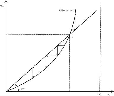
Figure 22.4 Saddle point equilibrium money balances in the Samuelson OLG Model.
The case where the elasticity of intertemporal substitution of consumption is lower than unity is depicted in figure 22.5. At some point, the offer curve for savings and money demand bends backward. If the offer curve crosses the 45° line on its backward-bending part at a slope that is greater than unity, the equilibrium at E is globally stable. This behavior implies that multiple converging paths lead to the equilibrium at E. The economy may thus display cyclical convergence to the equilibrium through a multitude of convergence paths.
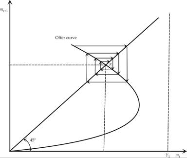
Figure 22.5 Multiple convergence paths for money balances in the Samuelson OLG model.
The possible existence of multiple convergent paths leading to a unique equilibrium at E is not the only problem of this model. The economy might have multiple equilibria and oscillate cyclically among them. An example of such multiple equilibria, due to Azariadis and Guesnerie [1986], is shown in figure 22.6.
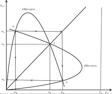
Figure 22.6 Multiple equilibria, sunspots, and cycles in the Samuelson OLG model.
Figure 22.6 depicts two possible equilibria. One is the saddle point at point E, and the second is an equilibrium with cycles between points A and B, which are defined by the intersection of the offer curve with its mirror image reflected through the 45° line. Which equilibrium will prevail will depend on the expectations of the young. Thus, periods of high prices will be followed by period of low prices, and vice versa.
Such equilibria that depend on self-fulfilling prophecies are examples of sunspots. Thus, if consumers believe that high prices will be followed by low prices, and vice versa, the economy will display high-low price cycles. If agents believe that prices will fall at a rate equal to the pure rate of time preference, then the equilibrium will be at E, with constantly falling prices and steady real money balances.
22.4.2 Other Models of Indeterminacy and Sunspots in Macroeconomics
Sunspot equilibria can be convergent or divergent, and a variety of examples can be constructed. In surveying the relevant literature, Benhabib and Farmer [1999] conclude that it
can be organized around three strands. First, there is work that uses models with indeterminate equilibria to explain the propagation mechanism of the business cycle. Second, there is a group of papers that uses indeterminacy to explain the monetary transmission mechanism, specifically the fact that prices are sticky, and third, there is work in growth theory that uses indeterminacy to understand why the per capita incomes of countries that are similar in their fundamentals nevertheless save and grow at different rates.
They go on to explain the ideas that underpin each of these strands and compare this literature to the more conventional approach.14
22.5