Optimal Dynamic Ramsey Taxation

The Barro [1979] model assumes but does not explicitly model the distortions implied by taxation. As we saw in the simple two-period intertemporal models of chapter 2, income taxes imply two main types of distortions.

The optimal choice of tax rates in an environment in which a representative household chooses among various consumption goods optimally was first studied formally by Ramsey [1927]. Dynamic versions of this problem have been studied by Lucas and Stokey [1983], Chamley [1986], Aiyagari et al. [2002], and Angeletos [2002]. Chari and Kehoe [1999] and Alesina and Passalacqua [2016] review this literature, which is known as the dynamic Ramsey approach to fiscal policy.

Consider an economy with an infinite number of periods and a large number of identical households. There is no uncertainty. The representative household has preferences of the form

where ρ is the pure rate of time preference, c_t+i is consumption in period t + i, l_t+i is labor supply in period t + i, and u and v are twice differentiable concave functions.

All households are initially endowed with k_t units of capital. Capital depreciates at a rate δ. In addition, households possess a technology that converts period t consumption goods into period t + 1 capital goods, and vice versa.

The economy has many competitive firms with a production technology that converts capital k and labor l into y units of consumption goods.

This function is quasi-concave and satisfies the usual properties of the neoclassical production function.

Households rent their labor services and capital goods to firms, in competitive factor markets. The returns to labor and capital are sequences of competitive real wages and real interest rates {w_t+i, r_t+i}.

The government can convert private goods into public goods one for one. The government is required to create a stream of public goods , i = 0, 1, …. The government needs to raise funds to make its purchases of public goods. It can find the funds through borrowing and lending at the sequence of competitive real interest rates {r_t+i}, levying linear taxes on labor income at rates , or levying linear taxes on capital income at rates .

The dynamic Ramsey problem consists of the government choosing the sequence of tax rates that maximizes the intertemporal utility function of the representative household, subject to the exogenous sequence of government purchases , the sequences of equilibrium private consumption and employment {c_t+i, l_t+i} resulting from the utility-maximizing choices of households and the profit-maximizing choices of firms, and the sequences of equilibrium real wages and real interest rates {w_t+i, r_t+i}.

One can show that the optimal sequence of tax rates satisfies³

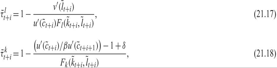
for i ≥ 1. The sequence is the optimal equilibrium sequence of private consumption, employment, and capital chosen by households and firms, given the optimal tax rates.

As discussed by Chari and Kehoe [1999], the optimal policy has the following two characteristics:

1. Capital income taxes must be high initially and then zero.

2. Tax rates on labor income should be constant.

The intuition behind the first characteristic is straightforward. A high capital income tax initially is optimal, because initial capital is predetermined. However, a positive capital income tax at date t means that the government is essentially taxing consumption in period t + 1 at a higher rate than consumption in period t. Hence, if the government maintains a positive long-run capital income tax rate, it is essentially taxing consumption at dates t + i at progressively higher rates, as i increases. As a result, the intertemporal distortion becomes progressively higher, and such an outcome is clearly suboptimal. Hence, capital income taxes must converge to zero.

In contrast, the second characteristic results because there is no reason to have time-varying static distortions between consumption and leisure, given the concavity of the utility functions. Hence, the optimal tax rate on labor income is positive and constant.

Tax smoothing is thus a characteristic of dynamic Ramsey taxation as well.

However, these results do not fully carry over to stochastic representative household models.

Lucas and Stokey [1983] consider a model with complete markets, no capital, exogenous Markov government expenditures, and state-contingent taxes and government debt. In this environment, optimal tax rates and government debt are not random walks, and the serial correlation of optimal taxes is tied closely to that of government purchases. Moreover, they find that taxes should be smooth, not by being random walks but by having a smaller variance than would be implied by a balanced budget. Thus, to some extent, the idea of tax smoothing holds but not in the extreme version of Barro [1979].

Aiyagari et al. [2002] reconsider the optimal taxation problem in an incomplete markets setting. They begin with the same economy as in Lucas and Stokey [1983] but allow only risk-free government debt. Under some restrictions on preferences and the quantities of risk-free claims that the government can issue and own, it is possible to recover Barro’s random walk characterization of optimal taxation.

However, by dropping the restriction on government asset holdings (or modifying preferences), one can generate different results, as, for example, in the model of Angeletos [2002], who considers noncontingent debt with varying maturities. The Angeletos model, although based on noncontingent debt, has implications similar to Lucas and Stokey [1983] in the presence of precommitment.

Additional complications arise in overlapping generations (OLG) models or other models with heterogeneous agents. For example, if households differ in their ability, but the government cannot directly observe or tax the ability of households and relies on their wage income instead, then additional distortions are introduced. Kocherlakota [2010] discusses a dynamic extension of the static Mirlees [1971] approach to this problem, as well as other extensions that rely on agent heterogeneity.

Another weakness of the dynamic Ramsey approach (but also other dynamic public finance approaches) is that without state-contingent government debt, dynamic optimal fiscal plans rely on precommitment. Such approaches have been shown to suffer from the time-inconsistency problem, meaning that at some point in time, the government may have an incentive to deviate from its preannounced ex ante optimal tax policy (Kydland and Prescott [1977], Calvo [1978]). For example, consider a policymaker (social planner) who, after a war (or a recession), is faced with tackling (reducing) the higher government debt that was accumulated during the war (or the recession). The ex ante optimal policy, on which the accumulation of debt was based, is to create primary surpluses by increasing tax rates after the war or the recession. However, ex post, the policymaker has at least three other options. First, to default on the debt. Second, to impose an extraordinary tax on the wealth of bondholders. Third, to generate unexpected inflation and monetize the debt. These options may appear ex post to imply smaller social costs than the rise in distortionary taxes. Thus, what was optimal before the accumulation of government debt may not appear optimal after government debt has accumulated. This is how the time-inconsistency problem arises. If the government succumbs to the temptation of the options of default, a capital levy, or monetization, it may lose reputation with bondholders and find it extremely difficult to borrow in the future. If the government sticks to the ex ante optimal policy, it does not lose reputation but may incur heavy social and political costs in trying to stabilize the debt that was accumulated through an increase in distortionary taxes. It may thus refrain from increasing future tax rates and follow one of the default options.

The solutions that have been proposed for the time-inconsistency problem resemble those that have been proposed for monetary policy. Binding budget rules and reform of political institutions can help constrain the freedom of governments to deviate from the ex ante optimal policy and thus can address the time inconsistency problem. Alesina and Passalacqua [2016] review the literature on this issue.

21.4