Physical and Human Capital with Imperfect Labor Markets
In this section, we analyze the implications of labor market frictions that lead to factor prices different from the ones we have used so far (in particular, in terms of the model of the last section, deviating from the competitive pricing formulea (10.31)).
The literature on labor market imperfections is vast and our purpose here is not to provide an overview. For this reason, we will adopt the simplest representation. In particular, imagine that the economy is identical to that described in the previous section, except that there is a measure 1 of firms as well as a measure 1 of individuals at any point in time, and each firm can only hire one worker. The production function of each firm is still given by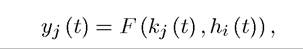
where yj (t) refers to the output of firm j, kj (t) is its capital stock (equivalently capital per worker, since the firm is hiring only one worker), and hi (t) is the human capital of worker i that the firm has matched with. This production function again satisfies Assumptions 1 and 2. The main departure from the models analyzed so far is that we now assume the following structure for the labor market:
(1) Firms choose their physical capital level irreversibly (incurring the cost R (t) kj (t), where R(t) is the market rate of return on capital), and simultaneously workers choose their human capital level irreversibly.
(2) After workers complete their human capital investments, they are randomly matched with firms. Random matching here implies that high human capital workers are not more likely to be matched with high physical capital firms.
(3) After matching, each worker-firm pair bargains over the division of output between themselves. We assume that they simply divide the output according to some prespecified rule, and the worker receives total earnings of
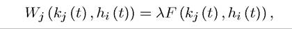
for some λ ∈ (0,1).
This is admittedly a very simple and reduced-form specification. Nevertheless, it will be sufficient to emphasize the main economic issues. A more detailed game-theoretic justification for a closely related environment is provided in Acemoglu (1996).
Let us next introduce heterogeneity in the cost of human capital acquisition by modifying (10.26) to
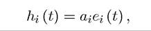
where ai differs across dynasties (individuals). A high-value of ai naturally corresponds to an individual who can more effectively accumulate human capital.
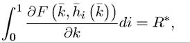
An equilibrium is defined similarly except that factor prices are no longer determined by (10.31). Let us start the analysis with the physical capital choices of firms. At the time each firm chooses its physical capital it is unsure about the human capital of the worker he will be facing. Therefore, the expected return of firm j can be written as

This expression takes into account that the firm will receive a fraction 1 — λ of the output produced jointly by itself and of worker that it is matched with. The integration takes care of the fact that the firm does not know which worker it will be matched with and thus we are taking the expectation of F (kj (t),hi (t)) over all possible human capital levels that are possible The last term is the cost of making irreversible capital
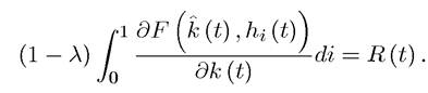
investment at the market price R (t). This investment is made before the firm knows which worker it will be matched with. The important observation is that the ob jective function in (10.38) is strict concave in kj (t) given the strict concavity of F (∙, ∙) from Assumption 1. Therefore, each firm will choose the same level of physical capital, k (t), such that
Now given this (expected) capital investment by firms, and following (10.33) from the previous section, each worker’s objective function can be written as:
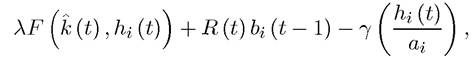
where we have substituted for the income mi (t) of the worker in terms of his wage earnings and capital income, and introduced the heterogeneity in human capital decisions.
This implies the following choice of human capital investment by a worker i: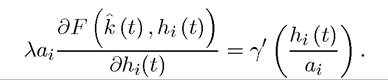
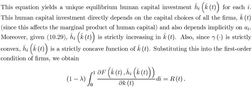
Finally, to satisfy market clearing in the capital market, the rate of return to capital, R (t), has to adjust, such that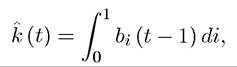
which follows from the facts that all firms choose the same level of capital investment and that the measure of firms is normalized to 1. This equation implies that in the closed economy version of the current model, capital per firm is fixed by bequest decisions from the previous period. The main economic forces we would like to emphasize here are seen more clearly when physical capital is not predetermined. For this reason, let us imagine that the economy in question is small and open, so that R (t) = R* is pinned down by international financial markets (the closed economy version is further discussed in Exercise 10.18). Under this assumption, the equilibrium level of capital per firm is determined by
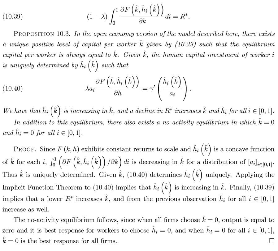
We have therefore obtained a simple characterization of the equilibrium in this economy with labor market frictions and physical and human capital investments. It is straightforward 403
to observe that there is underinvestment both in human capital and physical capital (this refers to the positive activity equilibrium; clearly, there is even a more severe underinvestment in the no-activity equilibrium). Consider a social planner wishing to maximize output (or one who could transfer resources across individuals in a lump-sum fashion). Suppose that the social planner is restricted by the same random matching technology, so that she cannot allocate workers to firms as she wishes.
A similar analysis to above implies that the social planner would also like each firm to choose an identical level of capital per firm, say k. However, this level of capital per firm will be different than in the competitive equilibrium and she will also choose a different relationship between human capital and physical capital investments. In particular, given k, she would make human capital decisions to satisfy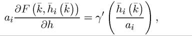
which is similar to (10.40), except that λ is absent from the left-hand side. This is because each worker considered only his share of output, λ, when undertaking his human capital investment decisions, while the social planner considers the entire output. Consequently, as long as λ < 1,
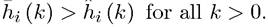
Similarly, the social planner would also choose a higher level of capital investment for each firm, in particular, to satisfy the equation
which differs from (10.39) both because now the term 1 — λ is not present on the left-hand side and also because the planner takes into account the differential human capital investment behavior of workers given by This discussion establishes the following result:
PROPOSITION 10.4. In the equilibrium described in Proposition 10.3, there is underinvestment both in physical and human capital.
More interesting than the underinvestment result is the imbalance in the physical to human capital ratio of the economy, which did not feature in the previous two environments we discussed. The following proposition summarizes this imbalance result in a sharp way:
PROPOSITION 10.5. Consider the positive activity equilibrium described in Proposition
10.3.
Output is equal to 0 if either λ = 0 or λ = 1. Moreover, there exists that
that maximizes output.
Proof. See Exercise 10.19. ?
Intuitively, different levels of λ create different types of “imbalances” between physical and human capital. A high level of λ implies that workers have a strong bargaining position, 404
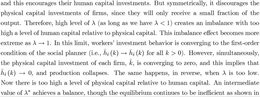
Proposition 10.5.
Physical-human capital imbalances can also increase the role of human capital in crosscountry income differences. In the current model, the proportional impact of a change in human capital on aggregate output (or on labor productivity) is greater than the return to human capital, since the latter is determined not by the marginal product of human capital, but by the bargaining parameter λ. The deviation from competitive factor prices, therefore, decouples the contribution of human capital to productivity from market prices.
At the root of the inefficiencies and of the imbalance effect in this model are pecuniary externalities. Pecuniary externalities refer to external effects that work through prices (not through direct technological spillovers). By investing more, workers (and symmetrically firms) increase the return to capital (symmetrically wages), and there is underinvestment because they do not take these external effects into consideration. Pecuniary external effects are also present in competitive markets (since, for example, supply affects price), but these are typically “second order,” because prices are such that they are equal to both the marginal benefit of buyers (marginal product of firms in the case of factors of production) and to the marginal cost of suppliers. The presence of labor market frictions causes a departure from this type of marginal pricing and is the reason why pecuniary externalities are not second order.
Perhaps even more interesting is the fact that pecuniary externalities in this model take the form of human capital externalities, meaning that greater human capital investments by a group of workers increase other workers’ wages. Notice that in competitive markets (without externalities) this does not happen. For example, in the economy analyzed in the last section, if a group of workers increase their human capital investments, this would depress the physical to human capital ratio in the economy, reducing wages per unit of human capital and thus the earnings of the rest of the workers. We will now see that the opposite may happen in the presence of labor market imperfections. To illustrate this point, let us suppose that there are two types of workers, a fraction of workers χ with ability ai and 1 — χ with ability a∙2 < aι.
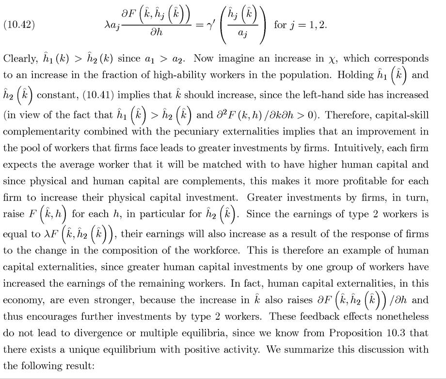
Using this specific structure, the first-order condition of firms, (10.39), can be written as 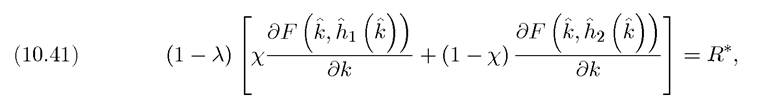 while the first-order conditions for human capital investments for the two types of workers take the form
Proposition 10.6. The positive activity equilibrium described in Proposition 10.3 exhibits human capital externalities in the sense that an increase in the human capital investments of a group of workers raises the earnings of the remaining workers.
10.7.