References and Literature

The empirical material presented in this chapter is largely standard and parts of it can be found in many books, though interpretations and exact emphases differ. Excellent in­troductions, with slightly different emphases, are provided in Jones’s (1998, Chapter 1) and Weil’s (2005, Chapter 1) undergraduate economic growth textbooks.

Much of the data used in this chapter comes from Summers-Heston’s Penn World tables (latest version, Summers, Heston and Aten, 2005). These tables are the result of a very careful study by Robert Summers and Alan Heston to construct internationally comparable price indices and internationally comparable estimates of income per capita and consumption. PPP adjustment is made possible by these data. Summers and Heston (1991) give a very lucid discussion of the methodology for PPP adjustment and its use in the Penn World tables. PPP adjustment enables us to construct measures of income per capita that are comparable 27

across countries. Without PPP adjustment, differences in income per capita across countries can be computed using the current exchange rate or some fundamental exchange-rate. There are many problems with such exchange-rate-based measures. The most important one is that they do not make an allowance for the fact that relative prices and even the overall price level differ markedly across countries. PPP-adjustment brings us much closer to differences in “real income” and “real consumption”.

In all figures and regressions, growth rates are computed as geometric averages. In par­ticular, the geometric average growth rate of output per capita y between date t and t + T is

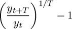
The geometric average growth rate is more appropriate to use in the context of income per capita than the arithmetic average, since the growth rate refers to “proportional growth”. It can be easily verified from this formula that if y_t+ι = (1+ g) y_t for all t, then g_t ∣ t = g.

Historical data are from various works by Angus Maddison (2001, 2005). While these data are not as reliable as the estimates from the Penn World tables, the general patterns they show are typically consistent with evidence from a variety of different sources. Nevertheless, there are points of contention. For example, as Figure 1.11 shows, Maddison’s estimates show a slow but relatively steady growth of income per capita in Western Europe starting in 1000. This is disputed by some historians and economic historians. A relatively readable account, which strongly disagrees with this conclusion, is provided in Pomeranz (2001), who argues that income per capita in Western Europe and the Yangtze Valley in China were broadly comparable as late as 1800. This view also receives support from recent research by Allen (2004), which documents that the levels of agricultural productivity in 1800 were comparable in Western Europe and China.

to a pattern in which there was already an income gap between Western Europe and China by the end of the 18th century.

The term takeoff I used in Section 1.4 is introduced in Walter Rostow’s famous book Stages of Economic Growth (1960) and has a broader connotation than the term “Industrial Revolution,” which economic historians typically use to refer to the process that started in Britain at the end of the 18th century (e.g., Ashton, 1968). Mokyr (1990) contains an excellent discussion of the debate on whether the beginning of industrial growth was due to a continuous or discontinuous change and, consistent with my emphasis here, concludes that this is secondary to the more important fact that the modern process of growth did start around this time.

There is a large literature on the “correlates of economic growth,” starting with Barro (1991), which is surveyed in Barro and Sala-i-Martin (2004) and Barro (1999). Much of this literature, however, interprets these correlations as causal effects, even when this is not war­ranted (see the further discussion in Chapters 3 and 4). Note that while Figure 1.15 looks at the relationship between the average growth of investment to GDP ratio and economic growth, Figure 1.16 shows the relationship between average schooling (not its growth) and economic growth. There is a much weaker relationship between growth of schooling and economic growth, which may be for a number of reasons; first, there is considerable measure­ment error in schooling estimates (see Krueger and Lindahl, 2000); second, as shown in in some of the models that will be discussed later, the main role of human capital may be to facilitate technology adoption, thus we may expect a stronger relationship between the level of schooling and economic growth than the change in schooling and economic growth (see Chapter 10); finally, the relationship between the level of schooling and economic growth may be partly spurious, in the sense that it may be capturing the influence of some other omitted factors also correlated with the level of schooling; if this is the case, these omitted factors may be removed when we look at changes.

The narrowing of income per capita differences in the world economy when countries are weighted by population is explored in Sala-i-Martin (2005). Deaton (2005) contains a critique of Sala-i-Martin’s approach. The point that incomes must have been relatively equal around 1800 or before, because there is a lower bound on real incomes necessary for the survival of an individual, was first made by Maddison (1992) and Pritchett (1996). Maddison’s estimates of GDP per capita and Acemoglu, Johnson and Robinson’s estimates based on urbanization confirm this conclusion.

The estimates of the density of income per capita reported above are similar to those used by Quah (1994, 1995) and Jones (1996). These estimates use a nonparametric Gaussian kernel. The specific details of the kernel estimates do not change the general shape of the densities. Quah was also the first to emphasize the stratification in the world income distrib­ution and the possible shift towards a “bi-modal” distribution, which is visible in Figure 1.3. He dubbed this the “Twin Peaks” phenomenon (see also Durlauf and Quah, 1994). Barro (1991) and Barro and Sala-i-Martin (1992) emphasize the presence and importance of condi­tional convergence, and argue against the relevance of the stratification pattern emphasized by Quah and others. The first chapter of Barro and Sala-i-Martin’s (2004) textbook contains a detailed discussion from this viewpoint.

The first economist to emphasize the importance of conditional convergence and conduct a cross-country study of convergence was Baumol (1986), but he was using lower quality data than the Summers-Heston data. This also made him conduct his empirical analysis on a selected sample of countries, potentially biasing his results (see De Long, 1991). Barro’s (1991) and Barro and Sala-i-Martin’s (1992) work using the Summers-Heston data has been instrumental in generating renewed interest in cross-country growth regressions.

The data on GDP growth and black real wages in South Africa are from Wilson (1972). Wages refer to real wages in gold mines. Feinstein (2004) provides an excellent economic history of South Africa. The implications of the British Industrial Revolution for real wages and living standards of workers are discussed in Mokyr (1993). Another example of rapid economic growth with falling real wages is provided by the experience of the Mexican economy in the early 20th century (see Gomez-Galvarriato, 1998). There is also evidence that during this period, the average height of the population might be declining as well, which is often associated with falling living standards, see Lopez Alonso and Porras Condy (2003).

There is a major debate on the role of technology and capital accumulation in the growth experiences of East Asian nations, particularly South Korea and Singapore. See Young (1994) for the argument that increases in physical capital and labor inputs explain almost all of the rapid growth in these two countries. See Klenow and Rodriguez-Clare (1996) and Hsieh (2001) for the opposite point of view.

The difference between proximate and fundamental causes will be discussed further in later chapters. This distinction is emphasized in a different context by Diamond (1996), though it is implicitly present in North and Thomas’s (1973) classic book. It is discussed in detail in the context of long-run economic development and economic growth in Acemoglu, Johnson and Robinson (2006). We will revisit these issues in greater detail in Chapter 4.