References and Literature
The AK model is a special case of Rebelo’s (1991), which was discussed in greater detail in Section 11.3 of this chapter. Solow’s (1965) book also discussed the AK model (naturally 435
with exogenous savings), but dismissed it as uninteresting.
A more complete treatment of sustained neoclassical economic growth is provided in Jones and Manuelli (1990), who show that even convex models (with production function is that satisfy Assumption 1, but naturally not Assumption 2) are consistent with sustained long-run growth. Exercise 11.4 is a version of the convex neoclassical endogenous growth model of Jones and Manuelli.Barro and Sala-i-Martin (2004) discuss a variety of two-sector endogenous growth models with physical and human capital, similar to the model presented in Section 11.2, though the model presented here is much simpler than similar ones analyzed in the literature.
Romer (1986) is the seminal paper of the endogenous growth literature and the model presented in Section 11.4 is based on this paper. Frankel (1962) analyzed a similar growth economy, but with exogenous constant saving rate. The importance of Romer’s paper stems not only from the model itself, but from two other features. The first is its emphasis on potential non-competitive elements in order to generate long-run economic growth (in this case knowledge spillovers). The second is its emphasis on the non-rival nature of knowledge and ideas. These issues will be discussed in greater detail in the next part of the book.
Another paper that has played a major role in the new growth literature is Lucas (1988), which constructs an endogenous growth model similar to that of Romer (1986), but with human capital accumulation and human capital externalities. Lucas’ model is also similar to the earlier contribution by Uzawa (1964). Lucas’s paper has played two major roles in the literature.
First, it emphasized the empirical importance of sustained economic growth and thus was instrumental in generating interest in the newly emerging endogenous growth models. Second, it emphasized the importance of human capital and especially of human capital externalities. Since the role of human capital was discussed extensively in Chapter 10, which also showed that the evidence for human capital externalities is rather limited, we focused on the Romer model rather than the Lucas model. It turns out that Lucas model also generates transitional dynamics, which are slightly more difficult to characterize than the standard neoclassical transitional dynamics. A version of the Lucas model is discussed in Exercise 11.20.11.7. Exercises
Exercise 11.1. Derive equation (11.14).
Exercise 11.2. Prove Proposition 11.2.
Exercise 11.3. Consider the following continuous time neoclassical growth model:
with aggregate production function
where A, B > 0.
(1) Define a competitive equilibrium for this economy.
(2) Set up the current-value Hamiltonian for an individual and characterize the necessary conditions for consumer maximization. Combine these with equilibrium factor market prices and derive the equilibrium path. Show that the equilibrium path displays non-trivial transitional dynamics.
(3) Determine the evolution of the labor share of national income over time.
(4) Analyze the impact of an unanticipated increase in B on the equilibrium path.
(5) Prove that the equilibrium is Pareto optimal.
Exercise 11.4. Consider the following continuous time neoclassical growth model:
with production function
(1) Define a competitive equilibrium for this economy.
(2) Set up the current-value Hamiltonian for an individual and characterize the necessary conditions for consumer maximization. Combine these with equilibrium factor market prices and derive the equilibrium path.
(3) Prove that the equilibrium is Pareto optimal in this case.
(4) Show that if σ ≤ 1, sustained growth is not possible.
(5) Show that if A and σ are sufficiently high, this model generates asymptotically sustained growth due to capital accumulation. Interpret this result.
(6) Characterize the transitional dynamics of the equilibrium path.
(7) What is happening to the share of capital in national income? Is this plausible? How would you modify the model to make sure that the share of capital in national income remains constant?
(8) Now assume that returns from capital are taxed at the rate τ. Determine the asymptotic growth rate of consumption and output.
Exercise 11.5. Derive equations (11.19) and (11.20).
Exercise 11.6. Consider the neoclassical growth model with Cobb-Douglas technology 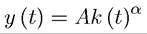 (expressed in per capita terms) and log preferences. Characterize the equilibrium path of this economy and show that as α → 1, equilibrium path approaches that of the baseline AK economy. Interpret this result.
Exercise 11.7. Consider the baseline AK model of Section 11.1 and suppose that two otherwise-identical countries have different taxes on the rate of return on capital. Consider the following calibration of the model where A = 0.15, δ = 0.05, ρ = 0.02, and θ = 3. Suppose that the first country has a capital income tax rate of τ = 0.2, while the second country has a tax rate of τ0 = 0.4. Suppose that the two countries start with the same level of income in 1900 and experience no change in technology or policies for the next 100 years. What will be the relative income gap between the two countries in the year 2000? Discuss this result and explain why you do (or do not) find the implications plausible.
EXERCISE 11.8. Prove that the necessary conditions for consumer optimization in Section 11.2 lead to the conditions enumerated in (11.25).
Exercise 11.9. Prove Proposition 11.3.
Exercise 11.10. Prove that the competitive equilibrium of the economy in Section 11.2, characterized in Proposition 11.3, is Pareto optimal and coincides with the solution to the optimal growth problem.
Exercise 11.11. Show that the rate of population growth has no effect on the equilibrium growth rate of the economies studied in Sections 11.1 and 11.2. Explain why this is. Do you find this to be a plausible prediction?
Exercise 11.12. * Show that in the model of Section 11.3, if the Cobb-Douglas assumption is relaxed, there will not exist a balanced growth path with a constant share of capital income in GDP.
Exercise 11.13. Consider the effect of an increase in α on the competitive equilibrium of the model in Section 11.3. Why does it increase the rate of capital accumulation in the economy? EXERCISE 11.14. Consider a variant of the model studied in Section 11.3, where the technology in the consumption-good sector is still given by (11.27), while the technology in the investment-good sector is modified to
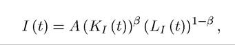
where β ∈ (α, 1). The labor market clearing condition requires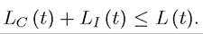 The
The
rest of the environment is unchanged.
(1) Define a competitive equilibrium.
(2) Characterize the steady-state equilibrium and show that it does not involve sustained growth.
(3) Explain why the long-run growth implications of this model differ from those of Section 11.3.
(4) Analyze the steady-state income differences between two economies taxing capital at the rates τ and τ0. What are the roles of the parameters α and β in determining these relative differences? Why do the implied magnitudes differ from those in the one-sector neoclassical growth model?
Exercise 11.15.
In the Romer model presented in Section 11.4, let be the growth rate of consumption and g* the growth rate of aggregate output. Show that
 '' is not feasible, while
 would violate the transversality condition.
 Exercise 11.16. Consider the Romer model presented in Section 11.4. Prove that the allocation in Proposition 11.5 satisfies the transversality condition. Prove also that there are no transitional dynamics in this equilibrium.
Exercise 11.17. Consider the Romer model presented in Section 11.4 and suppose that population grows at the exponential rate n. Characterize the labor market clearing conditions. Formulate the dynamic optimization problem of a representative household and show that any interior solution to this problem violates the transversality condition. Interpret this result.
Exercise 11.18. Consider the Romer model presented in Section 11.4. Provide two different types of tax/subsidy policies that would make the equilibrium allocation identical to the Pareto optimal allocation.
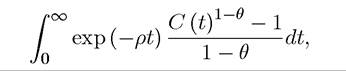
Exercise 11.19. Consider the following infinite-horizon economy in discrete time that admits a representative household with preferences at time t = O as
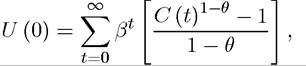
where C (t) is consumption, and β ∈ (0,1). Total population is equal to L and there is no population growth and labor is supplied inelastically. The production side of the economy consists of a continuum 1 of firms, each with production function

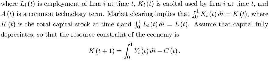
Assume also that labor-augmenting productivity at time t, A (t), is given by

(1) Explain (11.42) and why it implies a (non-pecuniary) externality.
(2) Define a competitive equilibrium (where all agents are price takers—but naturally not all markets are complete).
(3) Show that there exists a unique balanced growth path competitive equilibrium, where the economy grows (or shrinks) at a constant rate every period. Provide a
condition on F, β and θ such that this growth rate is positive, but the transversality condition is still satisfied.
(4) Argue (without providing the math) why any equilibrium must be along the balanced growth path characterized in part 3 at all points.
(5) Is this a good model of endogenous growth? If yes, explain why. If not, contrast it with what you consider to be better models.
EXERCISE 11.20. * Consider the following endogenous growth model due to Uzawa and Lucas. The economy admits a representative household and preferences are given by
where C (t) is consumption of the final good, which is produced as
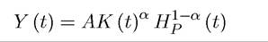
where K (t) is capital and H (t) is human capital, and Hp (t) denotes human capital used in production. The accumulation equations are as follows:
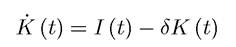
for capital and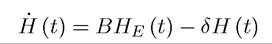
where He (t) is human capital devoted to education (further human capital accumulation), and the depreciation of human capital is assumed to be at the same rate as physical capital for simplicity (δ). The resource constraints of the economy are
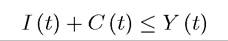
and
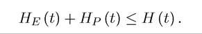
(1) Interpret the second resource constraint.
(2) Denote the fraction of human capital allocated to production by φ (t), and calculate the growth rate of final output as a function of φ (t) and the growth rates of accumulable factors.
(3) Assume that φ (t) is constant, and characterize the balanced growth path of the economy (with constant interest rate and constant rate of growth for capital and output). Show that in this balanced growth path, we have r* ? B — δ and the growth rate of consumption, capital, human capital and output are given by g* ? (B — δ — ρ) /θ. Show also that there exists a unique value of k* ? K/H consistent with balanced growth path.
(4) Determine the parameter restrictions to make sure that the transversality condition is satisfied.
(5) Now analyze the transitional dynamics of the economy starting with K/H different from k* [Hint: look at dynamics in three variables, k ? K/H, χ ? C/K and φ, and consider the cases α < θ and α ≥ θ separately].