Tax Smoothing and Government Debt Accumulation
The simplest explanations of government debt accumulation rely on a representative household economy. In such an economy, the theory of optimal taxation prescribes tax smoothing over time.
Because taxes are distortionary, they should not be changed to finance temporary or cyclical changes in the government budget. Debt financing should be used in the case of temporary rises in government purchases (such as during a war) or when tax receipts are temporarily low (such as during a recession); see Barro [1979] and Lucas and Stokey [1983]. Of course, permanent rises in government spending (such as those required for the expansion of the welfare state) ought to be financed through higher taxes, even if taxes are distortionary.21.1.1 The Barro Tax-Smoothing Model
Let us first explore the general intuition of the tax-smoothing result, using the model of Barro (1979). Assume that a government chooses a sequence of tax rates τt to finance a sequence of real primary government purchases  . Aggregate output Yt follows an exogenous stochastic process, as does the real interest rate rt. Taxes are distortionary, and the current aggregate distortion associated with a tax rate τt is given by

where f is a convex function that summarizes the various distortions associated with tax collection. Thus, f satisfies f′ > 0, f′′≥ 0.
At time t, the government has an inherited stock of real government debt Dt−1 from the end of period t − 1. As discussed in chapter 6, the intertemporal budget constraint of a solvent government is given by the requirement that at any time t, the expected present value of tax revenues must be greater than or equal to the expected present value of primary government expenditure, plus the initial level of government debt and its servicing cost.
In discrete time, this requirement can be written as
where Et is the mathematical expectations operator, conditional on information available in period t, and Rt+i denotes the real discount factor at time t + i. It is defined by

where rt+i is the market real interest rate in period t + i.
Assume that the government chooses a sequence of tax rates to minimize the expected present value of the distortions (21.1), subject to the intertemporal budget constraint (21.2), and taking the sequences of aggregate output and aggregate real government purchases as given. The Lagrange function for this problem is given by

where λt is the Lagrange multiplier.
From the first-order conditions for a minimum, it follows that

Equation (21.5) implies that

which implies that the optimal government tax policy is to keep the tax rate constant between periods. This is the basic tax-smoothing result. Under the optimal policy, there cannot be predictable changes in tax policy, and tax rates follow a random walk.
To derive the implications of tax smoothing for debts and deficits, let us consider the dynamic evolution of government debt. From the tax-smoothing first-order condition (21.6) and the government budget constraint (21.2), the tax rate at time t is determined by

The optimal distortionary tax rate is determined by two ratios.
The first is the stock of government debt inherited from period t− 1 plus its servicing cost, divided by the expected present value of aggregate output in period t. The second is the ratio of the expected present value of primary government purchases in period t to the expected present value of aggregate output in period t. The optimal tax rate is equal to the sum of those two ratios only. It is affected by current government purchases or current output only to the extent that these affect their respective present values.The evolution of government debt over time is determined by current government deficits. From the government budget constraint (21.2), the evolution of real government debt is determined by the following first-order difference equation:

Substituting (21.7) for τt in (21.8), after some rearrangement, we get
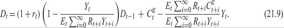
Consider first a temporary increase in Cg in period t, which leaves the expected present value of government purchases unchanged. This could be the effect of a war. It is clear from (21.9) that this increase would cause an increase in the current government deficit and an increase in government debt in period t. Thus, a temporary increase in government purchases causes an increase in government deficits and government debt, because the current optimal tax rate remains unchanged.
Consider next a temporary drop in current aggregate output Yt that leaves the expected present value of output unchanged. This could be the result of a recession. It is clear from (21.9) that this drop would also cause an increase in the current government deficit and current government debt, because, due to tax smoothing, the current optimal tax rate remains unchanged.
In contrast, a permanent change in either government purchases or output would not affect debt accumulation, because by (21.7), it would result in an increase in the current and expected future tax rates.
21.1.2 Steady State Implications of Tax Smoothing
To determine the steady state implications of the tax-smoothing model, consider a steady state in which the real interest rate is constant at r, output grows at an exogenously determined steady state growth rate g + n, and the same applies to real government purchases. The steady state growth rate is equal to the sum of the rate of technical progress g and population growth n. Assume that dynamic efficiency applies (i.e., that r > g + n).
The expected present value of output in the steady state is given by

The expected present value of government purchases is given by

Substituting (21.10) and (21.11) in (21.7), the optimal tax rate is given by

where dt = Dt/Yt is the government debt-to-output ratio, and  is the ratio of government purchases to output.
The optimal tax rate is equal to the ratio of government purchases to output plus that part of debt servicing which exceeds economic growth. Thus, the optimal tax rate is sufficient for financing not only permanent government purchases but also part of the servicing of government debt. A permanent increase in the ratio of government purchases to output thus brings about an equal permanent increase in the steady state optimal tax rate. A permanent increase in the government debt-to-output ratio also requires a permanent increase in steady state distortionary tax rates.
To find out how real government debt evolves under optimal tax smoothing, we can substitute (21.10) and (21.11) in (21.9).
Real government debt evolves according to
Thus, under the optimal tax-smoothing policy, in the steady state, real government debt is growing at the steady state growth rate g + n. As a result, the government debt-to-output ratio remains constant. Dividing (21.13) by real output, it is easy to see that

Thus, optimal tax policy of a solvent government stabilizes the government debt-to-output ratio in the steady state.
Therefore, this simple tax-smoothing model can explain the relative stability of tax rates, which only depend on the stock of inherited government debt and the present values of aggregate output and government purchases, as well as the positive effects of transitory shocks (such as wars and recessions) on government deficits and debts.
21.2