The Burden of High Government Deficits and Debt

Despite extensive research, the burden (i.e., social costs) of high government deficits and debt is not very well understood by macroeconomists. This is not unlike the case for the costs of inflation.

One reason is that the costs of deficits and government debt depend on the type of macroeconomic model one adopts. In representative household models with nondistortionary taxes, Ricardian equivalence holds, and sustainable government deficits and debts have zero real economic costs. In OLG models, high government debt results in lower savings and investment, lower growth rates, and lower steady state per capita income and consumption. In Keynesian models, higher government deficits during a recession help speed up the recovery and have posititive economic benefits. In models with distortionary taxation, higher government deficits and debts, even if sustainable, result in higher distortionary taxes, lower labor supply and employment, lower capital accumulation and growth, and lower steady state per capita income and consumption.

A second reason is that the costs of deficits and government debt also depend on the differential impact they have on the distribution of income. Welfare analysis is difficult to conduct, as it requires interpersonal and intergenerational comparisons of utility through a social welfare function.

A third reason is that in the presence of uncertainty, it is not straightforward to determine ex ante whether deficits are sustainable or unsustainable. Hence, to the extent that a high government debt is also deemed to be unsustainable, it is also associated with the possibility of a government debt crisis that will force a sudden stop to government borrowing, with possibly significant economic costs. Such a model of government debt crises is presented in the next section.

21.6 A Model of Government Debt Crises

In this section, we consider a simple two-period model of government debt crises. This model is due to Calvo [1988]. We focus on the question of what can cause a government debt crisis, in the sense that investors are not prepared to hold government bonds at a finite interest rate.

The model consists of two equilibrium conditions. The one equilibrium condition is the debt-holding condition. This condition requires the expected return on government debt to be equal to the return of a perfectly safe asset. The expected return is the probability of repayment, defined as one minus the expected default probability multiplied by the return on the government bond. The second equilibrium condition is a positive association of the probability of default with the level of government debt and the interest rate on government debt. Let us term this the debt-default condition.

21.6.1 The Calvo Model

Consider a two-period model. In period 0, the government wants to issue one-period bonds with a real value of D to finance its budget deficit. In period 1, which is the last period in the model, the government has to repay the debt, using the proceeds from its period 1 primary surplus S = T −C^g, where T is real tax revenue, assumed exogenous, and C^g is an exogenously determined amount of real government purchases.

The government offers investors a real interest rate r. Thus, in period 1, it will have to repay RD, where the interest factor R is defined by R = 1 + r. The primary surplus S in period 1 is uncertain and is a continuous random variable with a probability density function f(S) and a cumulative distribution function F(S).

If the primary surplus S in period 1 is higher than RD, the government repays the investors and, because this is the last period, returns the remaining revenue to households. If the primary surplus S is smaller that RD, the government cannot repay the full amount and defaults on its debt, returning the primary surplus to households.

Investors have access to a safe asset, which offers a safe rate of return r^*. Thus, the interest factor of the safe asset is equal to R^* = (1 + r^*).

To keep the model tractable, we thus make two simplifying assumptions. First, we assume that if the government cannot pay RD, then it pays nothing and defaults fully. Second, we assume that investors are risk neutral and that the rate of return of the safe asset R^*− 1 is independent of R and D.

In asset market equilibrium, the expected rate of return of government debt r = R − 1 should be equal to the rate of return of the safe asset, r^* = R^*− 1. If investors expect that government debt pays R with probability 1 − p^e, and zero with probability p^e, they will only buy government debt if (1 − p^e)R ≥ R^*. Arbitrage will ensure that the expected rate of return of government bonds will be driven down to the rate of return of the safe asset. Thus, with risk neutral investors, equilibrium in financial markets in period 0 will imply

The interest factor on government debt is thus given by

The higher the expected probability of default is, the higher the interest factor of government debt will be for a given interest factor of the safe asset. This equilibrium condition is depicted as the debt holding curve R = R^*/(1 − p^e) in figure 21.1. The interest factor of government debt R is a positive function of the expected probability of default p^e. As the expected probability of default tends to unity, R tends to infinity.

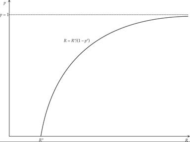
Figure 21.1 Expected default and the debt holding condition.

In fact, as a percentage of the interest factor R, the equilibrium risk premium on government debt is equal to the expected probability of default p^e. Solving (21.20) for p^e, we get

The second key relation of the model comes from the fact that the government defaults if and only if its primary surplus S in period 1 turns out to be lower than RD. Thus, the actual probability of default is equal to the probability that S is less than RD, or that S/D < R. Because F is assumed to be the cumulative distribution function of S, the actual probability of default is given by

Clearly, for a given D, the higher R is, the higher will be the actual probability of default, because the government requires a higher primary surplus to repay the higher interest charge on its debt.

The actual probability of default as a function of the interest factor R is depicted in figure 21.2 under two alternative assumptions about the density function f(S).

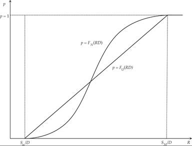
Figure 21.2 The actual probability of default and the cumulative distribution of the primary surplus.

The first assumption is that f(S) is the continuous uniform distribution, with support [S_m, S_M], where S_m is the minimum and S_M the maximum possible primary surplus in period 1. The shape of the cumulative distribution function under the assumption of a uniform density function is depicted as F_U(S) in figure 21.2. Between S_m/D and S_M/D, the cumulative distribution function rises at a constant rate from 0 to 1. Thus, if R < S_m/D, the probability of default p is equal to zero, and if R > S_M/D, the probability of default is equal to unity.

The second assumption is that f(S) is the truncated normal distribution, with support [S_m, S_M], where, again, S_m is the minimum and S_M the maximum possible primary surplus.

The shape of the cumulative distribution function under the assumption of a truncated normal density function is depicted as F_N(S) in figure 21.2. Between S_m/D and S_M/D, the cumulative distribution function rises, at an initially increasing and subsequently decreasing rate, from 0 to 1. Thus, if R < S_m/D, the probability of default p is equal to zero, and if R > S_M/D, the probability is equal to unity. In between, the probability of default lies between zero and one and is rising at an initially increasing and subsequently falling rate as the interest factor rises.

In fact, any symmetric bell-shaped continuous density function would have a cumulative distribution function with a shape similar to the one for the truncated normal distribution depicted in figure 21.2.

Rational expectations equilibrium requires that the expected probability of default is equal to the actual probability of default. Thus, both the debt holding condition (21.21) and the probability of default condition (21.22) must be satisfied simultaneously. Recall that the debt holding condition means that the higher the expected default probability is, the higher will be the interest rate required by investors. In contrast, the dependence of the probability of default on the uncertain primary surplus means that the higher the interest rate required by investors is, the higher the actual probability of default will be, given the distribution of the primary surplus. Because investors move first, a higher expected probability of default may result in a higher actual probability of default, stemming from the higher interest rate on government debt.

Figure 21.3 depicts the possible equilibria for the case of a uniform distribution. The figure shows the case of a low rate of return on the safe asset, in the sense that R^* < S_m/D. The economy depicted in figure 21.3, has three possible equilibria. One has a zero probability of default and a rate of return of government bonds equal to the rate of return of the safe asset r^*. The second, with an equilibrium at A, is characterized by a high probability of default and a high risk premium on government debt. The third has an equilibrium with a probability of default equal to unity and no government debt. This last equilibrium in fact implies a government debt crisis: The government cannot in this case find investors willing to hold government debt D at a finite interest rate.

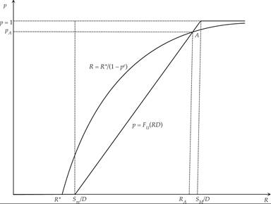
Figure 21.3 Determination of the interest factor and the probability of default for a low rate of return of the safe asset.

Which equilibrium will prevail depends on the prior expectations of investors about the probability of default. If investors believe that the default probability is zero, then the interest factor on government debt will be equal to R^*, and the default probability will indeed be zero. If investors believe that the default probability is high (say, p_A), then the interest factor on government debt will be at R_A, at a high premium over the safe asset R^*. The default probability will indeed be high in this case, and equal to p_A. Finally, if investors believe that the government will default with certainty (i.e., if p^e = 1), then the government will not be able to borrow at a finite interest rate, and a debt crisis will be the only equilibrium outcome.

Of the three equilibria, one is dynamically unstable in the sense that if investors adapt their expectations to close the gap between the expected and the actual probability of default, the economy will move toward the other two equilibria. In figure 21.3, this is equilibrium A with a high probability of default. If the expectations of investors lead to an interest factor slightly lower than R_A, then the expected probability of default will turn out to be higher than the actual probability of default. This would lead to a reduction in the expected probability of default, and the economy will converge to R^*. But if the expectations of investors lead to an interest factor slightly higher than R_A, then the expected probability of default will be lower than the actual probability of default. This would lead to a rise in the expected probability of default, and the economy will converge to a probability of default equal to unity and undergo a debt crisis. Thus, the only dynamically stable equilibria in this case are the equilibria with a zero and a unitary probability of default.

The equilibrium with a zero default probability and R = R^* is possible only if R^* < S_m/D. If R^* > S_m/D, this equilibrium is ruled out. The possible equilibria in this case are depicted in figure 21.4. Again there are three possible equilibria. The first is A, with a low probability of default and a rate of return of government bonds slightly higher than the rate of return of the safe asset r^*. The second equilibrium is B, with a high probability of default and a high risk premium on government debt. And the third is an equilibrium with a probability of default equal to unity and a government debt crisis. In the latter case, the government cannot find investors willing to hold government debt D at a finite interest rate. An analysis of the dynamic stability of the three equilibria suggests that the only dynamically stable equilibria are A and the equilibrium with a unitary probability of default; B is dynamically unstable. A similar analysis can be conducted using the truncated normal or any bell-shaped distribution instead of the uniform distribution.

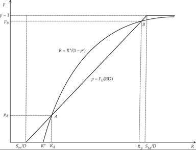
Figure 21.4 Determination of the interest factor and the probability of default for a high rate of return of the safe asset.

An important characteristic of this model is that, because of the multiplicity of equilibria, the probability of default depends not only on economic fundamentals (such as the size of real government debt and the probability distribution of the government primary surplus) but also on self-fulfilling expectations. If investors expect a zero or low probability of default, the actual probability of default will be zero or low. If investors expect a high probability of default, the actual probability of default will be high, and the government will have to pay a high interest premium. If the expected probability of default is equal to one, then the government will be unable to borrow at all, and a debt crisis will be the only equilibrium outcome.

21.6.2 Multiple Equilibria and Self-Fulfilling Prophecies

Because of nonlinearities in the model and the multiplicity of equilibria, small changes in the fundamentals can bring about large changes in equilibrium default probabilities and interest rates on government debt, or move the economy from one equilibrium to another.

We can draw four basic conclusions from this model. First, there are multiple equilibria. In the examples we have used, one equilibrium implies a zero or low probability of default and a low divergence of the interest rate on government debt from the safe rate. The second equilibrium implies a probability of default equal to unity and a failure of the government to borrow at any interest rate. A third intermediate equilibrium with a high probability of default exists as well, but it is dynamically unstable.

Second, in this model, the equilibrium that prevails depends on the expectations of investors. If investors expect a zero or low probability of default, the equilibrium will be characterized by a zero or low spread of the interest rate on government debt over the rate of the safe asset. If investors expect that the government will default with certainty, the government will be unable to borrow at any interest rate. Consequently, what equilibrium will prevail is to a large extent a self-fulfilling expectation or prophecy.

Third, small changes in the fundamentals can bring about large equilibrium changes and move us from one equilibrium to another. This is because even small changes to the fundamentals can cause large changes in expectations.

Fourth, when default occurs, it is unexpected. It is a jump from a low probability of default equilibrium to an equilibrium with a unitary probability of default.

The Calvo [1988] model can be extended to multiple time periods or to a monetary economy. In a monetary economy, instead of outright default, the government may choose to issue money to repay its debt, and default may take the form of unexpected high inflation. Again, there are multiple equilibria, such as an equilibrium with a low nominal interest rate and low inflation, or one with a high nominal interest rate and high inflation that wipes out government debt. With multiple time periods, it is of the utmost importance whether investors believe that other investors in the future will be willing to hold government debt.

This model and other stochastic default models interpret debt crises as crises of confidence that are caused by changes in the expectations of investors. These may take place because of changes in fiscal fundamentals, large or small. But they may also occur for other reasons that are purely expectational and not related to the fundamentals of fiscal policy.

21.7