The Misperceptions Theory and the Nonneutrality of Money

Summarize the fundamentals and implications of the misperceptions theory.

According to the classical model, prices do not remain fixed for any substantial period of time, so the horizontal short-run aggregate supply curve developed in Chapter 9 is irrelevant.

For money to be nonneutral, the relevant aggregate supply curve must not be vertical. In this section, we extend the classical model to incorporate the assump­tion that producers have imperfect information about the general price level and thus sometimes misinterpret changes in the general price level as changes in the relative prices of the goods that they produce. We demonstrate that the assump­tion that producers may misperceive the aggregate price level—the misperceptions theory—implies a short-run aggregate supply curve that isn't vertical. Unlike the short-run aggregate supply curve developed in Chapter 9, however, the short-run aggregate supply curve based on the misperceptions theory doesn't require the assumption that prices are slow to adjust. Even though prices may adjust instanta­neously, the short-run aggregate supply curve slopes upward, so money is non­neutral in the short run.

The misperceptions theory was originally proposed by Nobel laureate Milton Friedman and then was rigorously formulated by another Nobel laureate, Robert E. Lucas, Jr., of the University of Chicago.^[187] According to the misperceptions theory, the aggregate quantity of output supplied rises above the full-employment level, Y, when the aggregate price level, P, is higher than expected.

If you took a course in the principles of economics, you learned that supply curves generally slope upward, with higher prices leading to increased production. However, just as the demand curves for individual goods differ from the aggregate demand curve, the supply curves for individual goods differ from the aggregate supply curve. An ordinary supply curve relates the supply of some good to the price of that good relative to other prices. In contrast, the aggregate supply curve relates the aggregate amount of output produced to the general price level. Changes in the general price level can occur while the relative prices of individual goods remain unchanged.

To understand the misperceptions theory and why it implies an upward-sloping aggregate supply curve, let's think about an individual producer of a particular good, say bread. For simplicity, consider a bakery owned and operated by one per­son, a baker. The baker devotes all his labor to making bread and earns all his income from selling bread. Thus the price of bread is effectively the baker's nominal wage, and the price of bread relative to the general price level is the baker 's real wage. When the relative price of bread increases, the baker responds to this increase in his current real wage by working more and producing more bread. Similarly, when the price of bread falls relative to the other prices in the economy, the baker's current real wage falls and he decreases the amount of bread he produces.

But how does an individual baker know whether the relative price of bread has changed? To calculate the relative price of bread, the baker needs to know both the nominal price of bread and the general price level. The baker knows the nominal price of bread because he sells bread every day and observes the price directly. However, the baker probably is not as well informed about the general price level because he observes the prices of the many goods and services he might want to buy less frequently than he observes the price of bread.

Suppose that before he observes the current market price of bread, the baker expected an overall inflation rate of 5%. How will he react if he then observes that the price of bread increases by 5%? The baker reasons as follows: I expected the overall rate of inflation to be 5%, and now I know that the price of bread has increased by 5%. This 5% increase in the price of bread is consistent with what I had expected. My best estimate is that all prices increased by 5%, and thus I think that the relative price of bread is unchanged. There is no reason to change my output.

The baker's logic applies equally to suppliers of output in the aggregate. Suppose that all suppliers expected the nominal price level to increase by 5% and that in fact all prices do increase by 5%. Then each supplier will estimate that its relative price hasn't changed and won't change its output. Hence, if expected inflation is 5%, an actual increase in prices of 5% won't affect aggregate output.

For a change in the nominal price of bread to affect the quantity of bread pro­duced, the increase in the nominal price of bread must differ from the expected increase in the general price level. For example, suppose that the baker expected the general price level to increase by 5% but then observes that the price of bread rises by 8%. The baker then estimates that the relative price of bread has increased so that the real wage he or she earns from baking is higher. In response to the perceived increase in the relative price, he or she increases the production of bread.

Again, the same logic applies to the economy in the aggregate. Suppose that everyone expects the general price level to increase by 5%, but instead it actually increases by 8%, with the prices of all goods increasing by 8%.

Thus according to the misperceptions theory, the amount of output that produc­ers choose to supply depends on the actual general price level compared to the expected general price level. When the price level exceeds what was expected, pro­ducers are fooled into thinking that the relative prices of their own goods have risen, and they increase their output. Similarly, when the price level is lower than expected, producers believe that the relative prices of their goods have fallen, and they reduce their output. This relation between output and prices is captured by the equation where b is a positive number that describes how strongly output responds when the actual price level exceeds the expected price level. Equation (10.4) summarizes

FIGURE 10.7

The aggregate supply curve in the misperceptions theory

The misperceptions theory holds that, for a given value of the expected price level, P^e, an increase in the actual price level, P, fools producers into increasing output. This relationship between output and the price level is shown by the short-run aggregate supply (SRAS) curve. Along the SRAS curve, output equals Y when prices equal their expected level (P = P^e, at point E), output exceeds Y when the price level is higher than expected (P > P^e), and output is less than Y when the price level is lower than expected (P < P^e). In the long run, the expected price level equals the actual price level so that output equals Y.

the misperceptions theory by showing that output, Y, exceeds full-employment output, Y, when the price level, P, exceeds the expected price level, P^e.

To obtain an aggregate supply curve from the misperceptions theory, we graph Eq. (10.4) in Figure 10.7. Given full-employment output, Y, and the expected price level, P^e, the aggregate supply curve slopes upward, illustrating the relation between the amount of output supplied, Y, and the actual price level, P. Because an increase in the price level of ∆P increases the amount of the output supplied by ∆Y = b∆P, the slope of the aggregate supply curve is ∆P∕∆Y = 1/b. Thus the aggregate supply curve is steep if b is small and is relatively flat if b is large.

Point E helps us locate the aggregate supply curve. At E the price level, P, equals the expected price level, P^e, so that (from Eq. 10.4) the amount of output supplied equals full-employment output, Y. When the actual price level is higher than expected (P > P^e), the aggregate supply curve shows that the amount of output supplied is greater than Y; when the price level is lower than expected (P < P^e), output is less than Y.

The aggregate supply curve in Fig. 10.7 is called the short-run aggregate supply (SRAS) curve because it applies only to the short period of time that P^e remains unchanged. When P^e rises, the SRAS curve shifts up because a higher value of P is needed to satisfy Eq. (10.4) for given values of Y and Y. When P^e falls, the SRAS curve shifts down. In the long run, people learn what is actually happen­ing to prices, and the expected price level adjusts to the actual price level (P = P^e). When the actual price level equals the expected price level, no misperceptions remain and producers supply the full-employment level of output. In terms of Eq.

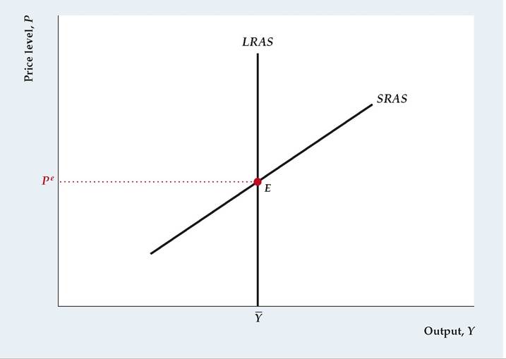
Monetary Policy and the Misperceptions Theory

Let's now reexamine the neutrality of money in the extended version of the classi­cal model based on the misperceptions theory. This framework highlights an important distinction between anticipated and unanticipated changes in the money supply: Unanticipated changes in the nominal money supply have real effects, but anticipated changes are neutral and have no real effects.

Unanticipated Changes in the Money Supply. Suppose that the economy is initially in general equilibrium at point E in Figure 10.8, where AD¹ intersects SRAS¹. Here, output equals the full-employment level, Y, and the price level and the expected price level both equal P₁. Suppose that everyone expects the money supply and the price level to remain constant but that the Fed unexpectedly and without publicity increases the money supply by 10%. A 10% increase in the money supply shifts the AD curve up and to the right, from AD¹ to AD 2, such that for a given Y, the price level on AD 2 is 10% higher than the price level on AD¹. With the expected price level equal to P₁, the SRAS curve remains unchanged, still passing through point E.

The increase in aggregate demand bids up the price level to the new equilib­rium level, P2, where AD 2 intersects SRAS¹ (point P). In the new short-run equilib­rium at P, the actual price level exceeds the expected price level and output exceeds Y. Because the increase in the money supply leads to a rise in output, money isn't neutral in this analysis.

The reason money isn't neutral is that producers are fooled. Each producer misperceives the higher nominal price of her output as an increase in its relative price, rather than as an increase in the general price level. Although output increases in the short run, producers aren't better off. They end up producing more than they would have if they had known the true relative prices.

The economy can't stay long at the equilibrium represented by point P because at P the actual price level, P2, is higher than the expected price level, P₁. Over time, people obtain information about the true level of prices and adjust their expectations accordingly. The only equilibrium that can be sustained in the long run is one in which people do not permanently underestimate or overesti­mate the price level so that the expected price level and the actual price level are equal. Graphically, when people learn the true price level, the relevant aggregate supply curve is the long-run aggregate supply (LRAS) curve, along which P always equals P^e. In Fig. 10.8 the long-run equilibrium is point H, the intersection of AD2 and LRAS. At H output equals its full-employment level, and the price level, P₃, is 10% higher than the initial price level, P₁. Becauseeveryone now expects the price level to be P₃, a new SRAS curve with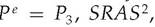passes

through H.

Thus according to the misperceptions theory, an unanticipated increase in the money supply raises output and isn't neutral in the short run. However, an unan­ticipated increase in the money supply is neutral in the long run, after people have learned the true price level.

FIGUREJ0.8

An unanticipated increase in the money supply

If we start from the initial equilibrium at point E, an unanticipated 10% increase in the money supply shifts the AD curve up and to the right, from AD¹ to AD², such that for a given Y, the price level on AD² is 10% higher than the price level on AD¹. The short-run equilibrium is located at point F, the intersection of AD² and the short-run aggregate supply curve SRAS¹, where prices and output are both higher than at point E. Thus an unanticipated change in the money supply isn't neutral in the short run. In the long run, people learn the true price level and the equilibrium shifts to point H, the intersection of AD² and the long-run aggregate supply curve LRAS. In the long-run equilibrium at H, the price level has risen by 10% but output returns to its full­employment level, Y, so that money is neutral in the long run. As expectations of the price level rise from P₁ to P₃, the SRAS curve also shifts up until it passes through H.

Anticipated Changes in the Money Supply. In the extended classical model based on the misperceptions theory, the effects of an anticipated money supply increase are different from the effects of a surprise money supply increase. Figure 10.9 illus­trates the effects of an anticipated money supply increase. Again, the initial general equilibrium point is at E, where output equals its full-employment level and the actual and expected price levels both equal P₁, just as in Fig. 10.8. Suppose that the Federal Reserve announces that it is going to increase the money supply by 10% and that the public believes this announcement.

As we have shown, a 10% increase in the money supply shifts the AD curve, from AD¹ to AD², where for each output level Y, the price level P on AD² is 10% higher than on AD¹. However, in this case the SRAS curve also shifts up. The reason is that the public's expected price level rises as soon as people learn of the increase in the money supply. Suppose that people expect—correctly— that the price level will also rise by 10% so that P^e rises by 10%, from P₁ to P₃. Then the new SRAS curve, SRAS², passes through point H in Fig. 10.9, where Y equals Y and both the actual and expected price levels equal P₃. The new equi­librium also is at H, where AD² and SRAS² intersect. At the new equilibrium, output equals its full-employment level, and prices are 10% higher than they were initially. The anticipated increase in the money supply hasn't affected out­put but has raised prices proportionally. Similarly, an anticipated drop in the money supply would lower prices but not affect output or other real variables. Thus anticipated changes in the money supply are neutral in the short run as well as in the long run. The reason is that, if producers know that increases in the nominal prices of their products are the result of an increase in the money supply and do not reflect a change in relative prices, they won't be fooled into increasing production when prices rise.

FIGUREJ0.9

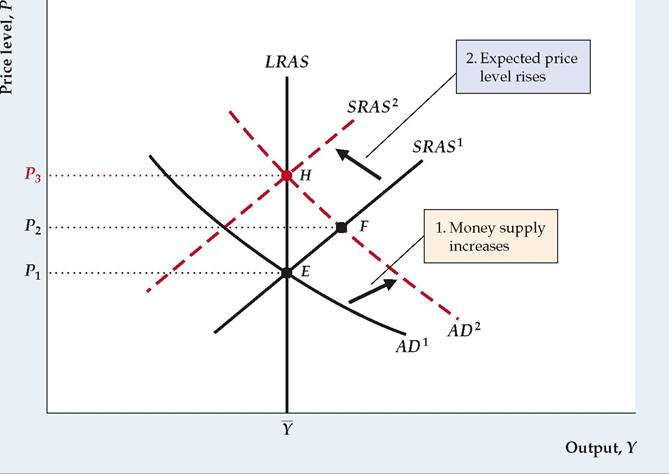
An anticipated increase in the money supply

The economy is in initial equilibrium at point E when the Fed publicly announces a 10% increase in the money supply. When the money supply increases, the AD curve shifts up by 10%, from AD¹ to AD 2. In addition, because the increase in the money supply is anticipated by the public, the expected price level increases by 10%, from P₁ to P₃. Thus the short-run aggregate supply curve shifts up from SRAS¹ to SRAS 2.

The new short-run equilibrium, which is the same as the long-run equilibrium, is at point H. At H output is unchanged at Y and the price level is 10% higher than in the initial equilibrium at E. Thus an anticipated increase in the money supply is neutral in the short run as well as in the long run.

Rational Expectations and the Role of Monetary Policy

In the extended classical model based on the misperceptions theory, unanticipated changes in the money supply affect output, but anticipated changes in the money supply are neutral. Thus if the Federal Reserve wanted to use monetary policy to affect output, it seemingly should use only unanticipated changes in the money supply. So, for example, when the economy is in recession, the Fed would try to use surprise increases in the money supply to raise output; when the economy is booming, the Fed would try to use surprise decreases in the money supply to slow the economy.

A serious problem for this strategy is the presence of private economic fore­casters and "Fed watchers" in financial markets. These people spend a good deal of time and effort trying to forecast macroeconomic variables such as the money supply and the price level, and their forecasts are well publicized. If the Fed began a pattern of raising the money supply in recessions and reducing it in booms, fore­casters and Fed watchers would quickly understand and report this fact. As a result, the Fed's manipulations of the money supply would no longer be unantici­pated, and the changes in the money supply would have no effect other than pos­sibly causing instability in the price level. More generally, according to the misperceptions theory, to achieve any systematic change in the behavior of out­put, the Fed must conduct monetary policy in a way that systematically fools the public. But there are strong incentives in the financial markets and elsewhere for people to try to figure out what the Fed is doing. Thus most economists believe that attempts by the Fed to surprise the public in a systematic way cannot be successful.

The idea that the Federal Reserve cannot systematically surprise the public is part of a larger hypothesis that the public has rational expectations. The hypothe­sis of rational expectations states that the public's forecasts of various economic variables, including the money supply, the price level, and GDP, are based on reasoned and intelligent examination of available economic data.^[188] (The evidence for rational expectations is discussed in "In Touch with Data and Research: Are Price Forecasts Rational?") If the public has rational expectations, it will eventually understand the Federal Reserve's general pattern of behavior. If expectations are rational, purely random changes in the money supply may be unanticipated and thus nonneutral. However, because the Fed won't be able to surprise the public systematically, it can't use monetary policy to stabilize output. Thus even if smooth­ing business cycles were desirable, according to the combination of the mispercep­tions theory and rational expectations, the Fed can't systematically use monetary policy to do so.

Propagating the Effects of Unanticipated Changes in the Money Supply. The misperceptions theory implies that unanticipated changes in the money supply are nonneutral because individual producers are temporarily fooled about the price level. However, money supply data are available weekly and price level data are reported monthly, suggesting that any misperceptions about monetary policy or the price level—and thus any real effects of money supply changes—should be quickly eliminated.

To explain how changes in the money supply can have real effects that last more than a few weeks, classical economists stress the role of propagation mecha­nisms. A propagation mechanism is an aspect of the economy that allows short­lived shocks to have relatively long-term effects on the economy.

An important example of a propagation mechanism is the behavior of inven­tories. Consider a manufacturing firm that has both a normal level of monthly sales and a normal amount of finished goods in inventory that it tries to main­tain. Suppose that an unanticipated rise in the money supply increases aggregate demand and raises prices above their expected level. Because increasing produc­tion sharply in a short period of time is costly, the firm will respond to the increase in demand partly by producing more goods and partly by selling some finished goods from inventory, thus depleting its inventory stocks below their normal level.

Next month suppose that everyone learns the true price level and that the firm's rate of sales returns to its normal level. Despite the fact that the monetary shock has passed, the firm may continue to produce for a while at a higher than normal rate. The reason for the continued high level of production is that besides meeting its normal demand, the firm wants to replenish its inventory stock. The need to rebuild inventories illustrates a propagation mechanism that allows a short-lived shock (a monetary shock, in this case) to have a longer-term effect on the economy.

In Touch with Data and Research

Are Price Forecasts Rational?

Most classical economists assume that people have rational expectations about economic variables; that is, people make intelligent use of available information in forecasting variables that affect their economic decisions. The rational expecta­tions assumption has important implications. For example, as we have demon­strated, if monetary nonneutrality is the result of temporary misperceptions of the price level and people have rational expectations about prices, monetary policy is not able to affect the real economy systematically.

The rational expectations assumption is attractive to economists—including many Keynesian as well as classical economists—because it fits well economists' presumption that people intelligently pursue their economic self-interests. If peo­ple's expectations aren't rational, the economic plans that individuals make won't generally be as good as they could be. But the theoretical attractiveness of ratio­nal expectations obviously isn't enough; economists would like to know whether people really do have rational expectations about important economic variables.

The rational expectations idea can be tested with data from surveys, in which people are asked their opinions about the future of the economy. To illustrate how such a test would be conducted, suppose that we have data from a survey in which people were asked to make a prediction of the price level one year in the future. Imagine that this survey is repeated each year for several years. Now sup­pose that, for each individual in the survey, we define

P_t^e = the individual's forecast, made in year t — 1, of the price level in year t. Suppose also that we let P_t represent the price level that actually occurs in year t. Then the individual's forecast error for year t is the difference between the actual price level and the individual 's forecast:

If people have rational expectations, these forecast errors should be unpre­dictable random numbers. However, if forecast errors are consistently positive or negative—meaning that people systematically tend to underpredict or overpre­dict the price level—expectations are not rational. If forecast errors have a system­atic pattern—for example, if people tend to overpredict the price level when prices have been rising in the recent past—again, expectations are not rational.

Early statistical studies of price level forecasts made by consumers, journal­ists, professional economists, and others tended to reject the rational expecta­tions theory. These studies, which were conducted in the late 1970s and early 1980s, followed the period in which inflation reached unprecedented levels, in part because of the major increases in oil prices and expansionary monetary policy in 1973-1974 and in 1979. It is perhaps not surprising that people found forecasting price changes to be unusually difficult during such a volatile period.

Later studies of price level forecasts have been more favorable to the rational expectations theory. Michael Keane and David Runkle^[189] of the Federal Reserve

Bank of Minneapolis studied the price level forecasts of a panel of professional forecasters that has been surveyed by the American Statistical Association and the National Bureau of Economic Research since 1968. They found no evidence to refute the hypothesis that the professional forecasters had rational expectations. In another article, Dean Croushore^[190] of the University of Richmond analyzed a variety of forecasts made not only by economists and forecasters but also by mem­bers of the general public, as reported in surveys of consumers. Croushore found that the forecasts of each of these groups were broadly consistent with rational expectations, although there appeared to be some tendency for expectations to lag behind reality in periods when inflation rose or fell sharply.