The Representative Household

When we say that an economy admits a representative household, this means that the pref­erence (demand) side of the economy can be represented as if there were a single household making the aggregate consumption and saving decisions (and also the labor supply decisions when these are endogenized) subject to a single budget constraint.

Let us start with the simplest case that will lead to the existence of a representative household. Suppose that each household is identical, i.e., it has the same discount factor β, the same sequence of effective labor endowmentsand the same instantaneous

utility function

where u :is increasing and concave and Ci (t) is the consumption of household

i.

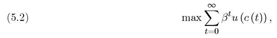
where β ∈ (0,1) is the common discount factor of all the households, and c (t) is the con­sumption level of the representative household.

The economy described so far admits a representative household rather trivially; all house­holds are identical. In this case, the representative household’s preferences, (5.2), can be used not only for positive analysis (for example, to determine what the level of savings will be), but also for normative analysis, such as evaluating the optimality of different types of equilibria.

Often, we may not want to assume that the economy is indeed inhabited by a set of identical households, but instead assume that the behavior of the households can be modeled as if it were generated by the optimization decision of a representative household. Naturally, this would be more realistic than assuming that all households are identical. Nevertheless, 182

this is not without any costs. First, in this case, the representative household will have positive meaning, but not always a normative meaning (see below). Second, it is not in fact true that most models with heterogeneity lead to a behavior that can be represented as if it were generated by a representative household.

In fact most models do not admit a representative household. To illustrate this, let us consider a simple exchange economy with a finite number of commodities and state an important theorem from general equilibrium theory. In preparation for this theorem, recall that in an exchange economy, we can think of the object of interest as the excess demand functions (or correspondences) for different commodities. Let these be denoted by x (p) when the vector of prices is p.

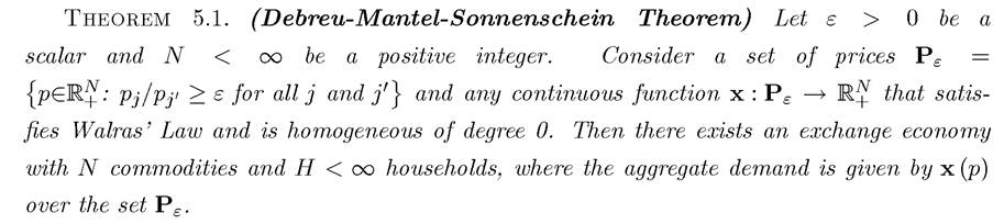
PROOF. See Debreu (1974) or Mas-Colell, Winston and Green (1995), Proposition 17.E.3.

?

This theorem states the following result: the fact that excess demands come from the optimizing behavior of households puts no restrictions on the form of these demands. In particular, x (p) does not necessarily possess a negative-semi-definite Jacobian or satisfy the weak axiom of revealed preference (which are requirements of demands generated by individ­ual households). This implies that, without imposing further structure, it is impossible to derive the aggregate excess demand, x (p), from the maximization behavior of a single house­hold. This theorem therefore raises a severe warning against the use of the representative household assumption.

Nevertheless, this result is partly an outcome of very strong income effects. Special but approximately realistic preference functions, as well as restrictions on the distribution of income across individuals, enable us to rule out arbitrary aggregate excess demand functions. To show that the representative household assumption is not as hopeless as Theorem 5.1 suggests, we will now show a special and relevant case in which aggregation of individual preferences is possible and enables the modeling of the economy as if the demand side was generated by a representative household.

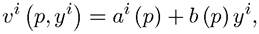
To prepare for this theorem, consider an economy with a finite number N of commodities and recall that an indirect utility function for household i, Vi (p, yⁱ), specifies the household’s (ordinal) utility as a function of the price vector p = (pχ,...,pv) and the household’s income yⁱ. Naturally, any indirect utility function Vi (p,yⁱ) has to be homogeneous of degree 0 in p and y.

Theorem 5.2. (Gorman's Aggregation Theorem) Consider an economy with a finite number N < ∞ of commodities and a set H of households. Suppose that the preferences of householdcan be represented by an indirect utility function of the form

(5.3)

then these preferences can be aggregated and represented by those of a representative house­hold, with indirect utility

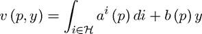
where ó ? f yⁱdi is aggregate income.

Proof. See Exercise 5.3.

?

This theorem implies that when preferences admit this special quasi-linear form, we can represent aggregate behavior as if it resulted from the maximization of a single household. This class of preferences are referred to as Gorman preferences after Terrence Gorman, who was among the first economists studying issues of aggregation and proposed the special class of preferences used in Theorem 5.2. The quasi-linear structure of these preferences limits the extent of income effects and enables the aggregation of individual behavior. Notice that instead of the summation, this theorem used the integral over the set H to allow for the possibility that the set of households may be a continuum. The integral should be thought of as the “Lebesgue integral,” so that when H is a finite or countable set,is indeed equivalent to the summationNote also that this theorem is stated for an economy with a finite number of commodities. This is only for simplicity, and the same result can be generalized to an economy with an infinite or even a continuum of commodities.

Note also that for preferences to be represented by an indirect utility function of the Gorman form does not necessarily mean that this utility function will give exactly the indirect utility in (5.3). Since in basic consumer theory a monotonic transformation of the utility function has no effect on behavior (but affects the indirect utility function), all we require is that there exists a monotonic transformation of the indirect utility function that takes the form given in (5.3).

Another attractive feature of Gorman preferences for our purposes is that they contain some commonly-used preferences in macroeconomics. To illustrate this, let us start with the following example:

EXAMPLE 5.1. (Constant Elasticity of Substitution Preferences) A very common class of preferences used in industrial organization and macroeconomics are the constant elasticity of substitution (CES) preferences, also referred to as Dixit-Stiglitz preferences after the two economists who first used these preferences. Suppose that each household denoted by has total income y^l and preferences defined over j = 1,..., N goods given by

(5.4)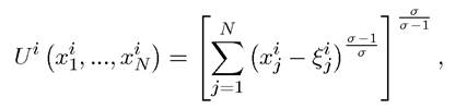

where σ ∈ (0, ∞) and ξj ∈ [—ξ, ξ] is a household specific term, which parameterizes whether the particular good is a necessity for the household. For example,I may mean that household i needs to consume a certain amount of good j to survive. The utility function

(5.4) is referred to as constant elasticity of substitution (CES), since if we define the level of consumption of each good as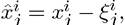the elasticity of substitution between any two Xj

andwould be equal to σ.

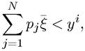
Each consumer faces a vector of prices p=(pι,...,pN), and we assume that for all i,

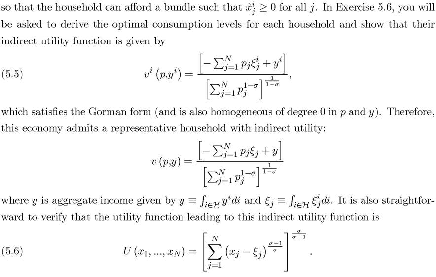
We will see below that preferences closely related to the CES preferences will play a special role not only in aggregation but also in ensuring balanced growth in neoclassical growth models.

It is also possible to prove the converse to Theorem 5.2. Since this is not central to our focus, we state this result in the text rather than stating and proving it formally. The essence of this converse is that unless we put some restrictions on the distribution of income across households, Gorman preferences are not only sufficient for the economy to admit a representative household, but they are also necessary. In other words, if the indirect utility functions of some households do not take the Gorman form, there will exist some distribution of income such that aggregate behavior cannot be represented as if it resulted from the maximization problem of a single representative household.

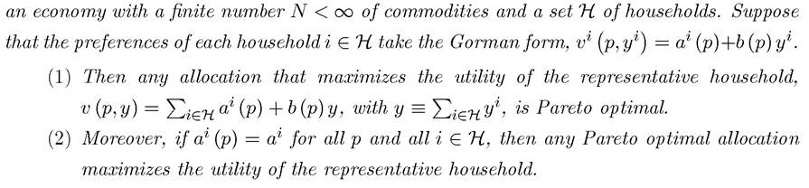
In addition to the aggregation result in Theorem 5.2, Gorman preferences also imply the existence of a normative representative household. Recall that an allocation is Pareto optimal if no household can be made strictly better-off without some other household being made worse-off (see Definition 5.2 below). We then have:

Theorem 5.3. (Existence of a Normative Representative Household) Consider

Proof. We will prove this result for an exchange economy. Suppose that the economy has a total endowment vector ofThen we can represent a Pareto optimal

allocation as:

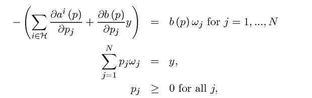
subject to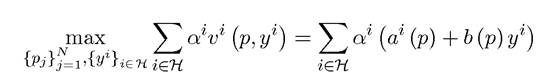

whereare nonnegative Pareto weights with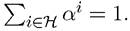The first set of constraints

use Roy’s identity to express the total demand for good j and set it equal to the supply of good j, which is the endowmentThe second equation makes sure that total income in 186

the economy is equal to the value of the endowments. The third set of constraints requires that all prices are nonnegative.

Now compare the above maximization problem to the following problem:

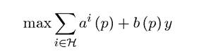
subject to the same set of constraints. The only difference between the two problems is that in the latter each household has been assigned the same weight.

be a solution to the second problem. By definition it is also a solution to the first problem with αⁱ = α, and therefore it is Pareto optimal, which establishes the first part of the theorem.

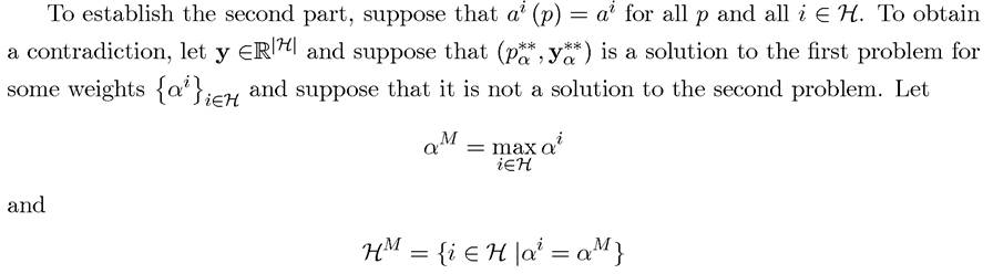
be the set of households given the maximum Pareto weight.be a solution to the

second problem such that

(5.7)

Note that such a solution exists since the objective function and the constraint set in the second problem depend only on the vector

Since, by definition, (pjj*, y‰*) is in the constraint set of the second problem and is not a solution, we have

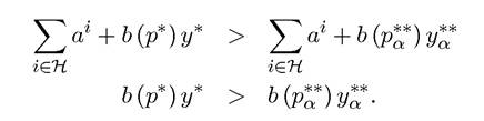
The hypothesis that it is a solution to the first problem also implies that

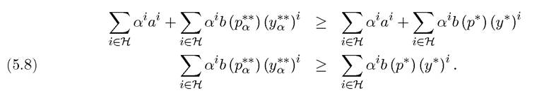
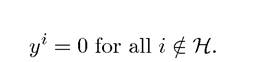
Then, it can be seen that the solutionto the Pareto optimal allocation problem satisfies y^l = 0 for any iIn view of this and the choice of (p*,y*) in (5.7), equation 187

(5.8) implies

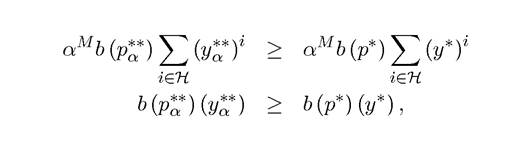
which contradicts equation (5.8), and establishes that, under the stated assumptions, any Pareto optimal allocation maximizes the utility of the representative household. ?

5.3.