The Solow Growth Model

To account for the process of economic growth, the Solow model focuses on the determination of three main aggregate endogenous variables: total output Y, total physical stock K, and aggregate consumption C.

Thus, the rate of growth in the number of employees is equal to the population growth rate n and is considered exogenous. The rate of growth in the efficiency of labor is equal to the rate of exogenous technical progress g.

The model explains the level and rate of growth of output and physical capital as functions of these exogenous factors (n and g), the savings rate s (which is also considered exogenous), total factor productivity, and the exogenous rate of depreciation of capital δ. Once the capital stock, output, consumption, and investment are determined, one can derive the real interest rate r (renumeration of capital) and real wages w (remuneration of labor), as these depend on the ratio of capital to total labor efficiency. Obviously, all endogenous variables are determined simultaneously in a dynamic general equilibrium.

3.1.1 The Neoclassical Production Function

A key assumption that differentiates the Solow model from the models of economic growth that preceded it is the neoclassical production function. This function, as we discussed in chapter 2, implies a positive but finite elasticity of substitution between factors of production. Thus, at each point in time t, the economy is assumed to possess a stock of capital, number of employees, and labor efficiency that are combined to produce output through this production function.

where A is a positive constant denoting total factor productivity, and F is a continuous, twice differentiable quasi-concave function. We assume, as in chapter 2, that F is characterized by positive but diminishing returns to each factor of production but constant returns to scale. Hence, F is also a linearly homogeneous function.

Growth models that preceded the Solow model, such as the Harrod [1939]–Domar [1946] model, were based on a fixed proportions production function without the possibility of substitution between capital and labor. Such a production function was also used by Leontieff [1941] and is called the Leontieff production function. However, these earlier models did not necessarily imply covergence to a balanced growth path because of the lack of substitutability between capital and labor.

It is worth noting the following five characteristics of the neoclassical production function. First, time t enters the production function solely through the factors of production K(t) and h(t)L(t). Output can change over time only through changes in the quantity or efficiency of factors of production.

Second, technical progress is assumed to increase only the efficiency of labor h(t). This is called labor augmenting technical progress, or Harrod neutral technical progress.

Third, the production function is characterized by constant returns to scale. Multiplying all factors of production by any nonnegative real number multiplies the scale of production by the same nonnegative real number. Thus, (3.1) satisfies

for any μ ≥ 0. Because of the assumption of constant returns to scale, the production function can be rewritten as

where y = Y/hL is output per efficiency unit of labor, k = K/hL is capital per efficiency unit of labor, and f(k) = F(k, 1) is the production function per efficiency unit of labor.

Fourth, it is assumed that the production function has the following properties:

The marginal product of capital per efficiency unit of labor is positive but declining. The production function in intensive form, with these additional assumptions, is depicted in figure 3.1.

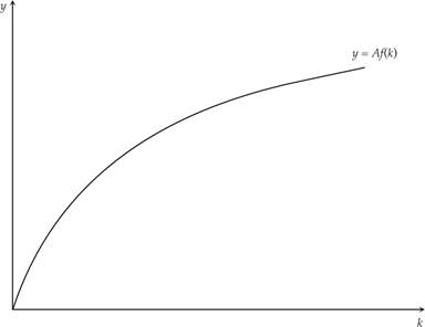
Figure 3.1 The production function in intensive form.

Fifth, it is assumed that

These final assumptions are called the Inada conditions. The Inada conditions ensure that the marginal product of capital is very high when capital intensity is low, and very low when capital intensity is high. These conditions are necessary and sufficient in order to prove the global uniqueness of the balanced growth path.²

3.1.2 The Cobb-Douglas Production Function

A particular production function that is often used in the theory of growth, but also more generally in macroeconomics, is the Cobb-Douglas production function. As already discussed in chapter 2, it takes the form

where A > 0, 0 < α < 1, α is the elasticity of production with respect to capital, and 1 − α is the corresponding elasticity with respect to labor.

The Cobb-Douglas production function in intensive form is given by

One can easily confirm that the Cobb-Douglas production function (3.3) satisfies all the assumptions we have made about the neoclassical production function.

In addition, for the Cobb-Douglas production function, labor augmenting technical progress (Harrod neutral) does not differ from capital augmenting technical progress, or technical progress that augments both factors (Hicks neutral). The reason is that in the Cobb-Douglas production function, the factors of production enter multiplicatively, and thus, it does not matter which of the factors of production is multiplied by technical progress.³

3.1.3 Population Growth and Technical Progress

We analyze the Solow model in continuous time, assuming that t is a continuous variable, where t ∈ [0, ∞).⁴ Assume that the number of employees is a constant fraction of total population and grows continuously at a constant, exogenous rate of population growth n. Thus, employment evolves over time according to

where L(0) is the number of employees at time 0, and e is the base of natural logarithms. Also assume that the efficiency of labor also grows continuously at a constant exogenous rate of technical progress g:

where h(0) is the efficiency of labor at time 0.

From (3.5) and (3.6), it follows that

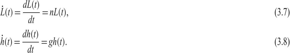
A dot over a variable denotes its first derivative with respect to time (i.e., its change over time).⁵

3.1.4 Savings, Capital Accumulation, and Economic Growth

The output produced accrues to households as income, which is either consumed or saved. In the Solow model, the share of income which is saved and invested in any instant is assumed to be an exogenous parameter, denoted by s.

Aggregate consumption C, is thus given by

The demand for total output consists of consumption plus gross investment:

where I(t) is gross investment.

Gross investment consists of additions to the capital stock plus replacement investment and is given by

where 0 < δ < 1 is the rate of depreciation of the capital stock, assumed to be a constant exogenous parameter. Thus, δ is the instantaneous rate at which the capital stock declines over time because of wear and tear.

Substituting the consumption function (3.9) and the definition of gross investment (3.11) in the equilibrium condition (3.10), we get

Solving (3.12) for the change in the capital stock yields

From (3.13), the accumulation of capital is determined by the difference between savings and replacement investment. To the extent that savings is higher than replacement investment, the capital stock grows over time. If savings is lower than replacement investment, the capital stock is reduced over time.

Dividing (3.13) through by hL and taking into account that L grows at rate n and h grows at rate g, we get

which is the capital accumulation equation expressed in efficiency units of labor. To the extent that savings per efficiency unit of labor is higher than the investment required to keep capital per efficiency unit of labor constant, capital per efficiency unit of labor grows over time. In the opposite case, it declines over time.

Using the production function in intensive form, (3.2), to replace y in (3.14), we get

The nonlinear differential equation (3.15) is the key equation determining the accumulation of capital in the Solow model.

3.1.5 The Balanced Growth Path and the Convergence Process

Given that the aggregate labor force, in efficiency terms, is increasing at an exogenous rate n + g, and that a fraction δ of the capital stock needs to be replaced at every moment due to depreciation, the investment required to keep the capital stock per efficiency unit of labor constant is given by (n + g + δ)k. This we denote as steady state investment.

Steady state capital per efficiency unit of labor is thus determined by the condition that

Denote by k^* the capital stock per efficiency unit of labor k that satisfies (3.16). One can easily deduce that k^* is constant and independent of time. It defines the so-called balanced growth path or steady state of the model, as all other steady state variables in this model depend on k^*.

On the steady state (or balanced growth) path, the capital stock, output, consumption, and investment per efficiency unit of labor are constant. The per capita steady state capital stock, output, consumption, and investment are of course not constant, as they are all growing at the exogenous rate of technical progress g. The aggregate steady state capital stock, output, consumption, and investment are growing at the rate g + n, which is the sum of the rate of population growth and the rate of technical progress.

The determination of k^* and the dynamic adjustment of k toward k^* are depicted in figure 3.2. The straight line depicts steady state investment (n + g + δ)k. The curved line sAf(k) depicts current savings and investment. At the point k^*, current savings and investment are equal to steady state savings and investment. Also depicted in Figure 3.2 is the production function in intensive form Af(k), which relates output per efficiency unit of labor to capital per efficiency unit of labor.

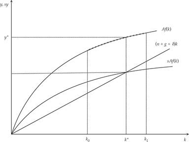
Figure 3.2 Equilibrium in the Solow model.

To the left of k^*, current investment is higher than steady state investment, and k is increasing over time. To the right of k^*, current investment is lower than steady state investment, and k is declining over time. The equilibrium at k^* is unique and globally stable. Irrespective of initial conditions, the economy converges to k^*, which is the steady state capital stock per efficiency unit of labor.

Exercise 3.1 Assuming a Cobb-Douglas production function, as in (3.4), derive the steady state capital stock per efficiency unit of labor in the Solow model, as represented in (3.16). Also derive steady state output and consumption per efficiency unit of labor. How do these steady state variables depend on the savings rate s, total factor productivity A, the rate of technical progress g, the rate of growth of population n, and the depreciation rate δ? Discuss.

3.1.6 The Rate of Growth of Capital and Output

To examine the behavior of the growth rate of capital per efficiency unit of labor in the Solow model, we can divide both sides of equation (3.15) by k(t). We then find that the growth rate of capital per efficiency unit of labor is given by

The growth rate of capital (per efficiency unit of labor) in the Solow model depends on the difference of the average product of capital, multiplied by the savings rate, from the sum of population growth, the rate of technical progress and the depreciation rate. If savings per unit of capital exceed steady state investment per unit of capital, then capital per efficiency unit of labor displays positive growth, as the capital stock increases at a rate higher than n + g. In the opposite case, capital per efficiency unit of labor displays negative growth, as the capital stock either falls or grows at a rate lower than n + g. In the steady state, capital per efficiency unit of labor is constant, as the capital stock grows at a rate equal to n + g. The determination of the growth rate is depicted in figure 3.3.

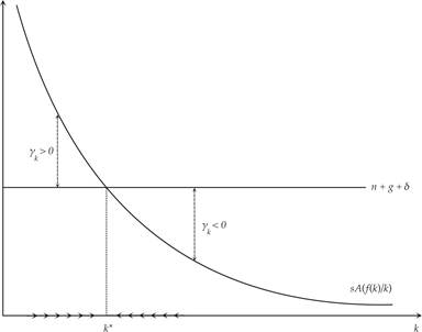
Figure 3.3 Determination of the growth rate.

The downward sloping curve depicts savings per unit of capital. As capital per efficiency unit of labor increases, savings per unit of capital fall, because the marginal and average product of capital is decreasing. This curve approaches infinity as capital tends to zero, and it approaches zero as capital tends to infinity, because of the Inada conditions. The straight line n + g + δ depicts steady state investment per unit of capital. It is the investment required to keep capital per efficiency unit of labor constant. Because of the Inada conditions, the two curves intersect at a positive capital stock per efficiency unit of labor, which is the steady state capital stock k^*. To the left of k^*, the growth rate of k is positive and declining, and to the right of k^*, the growth rate of k is positive and increasing. At k^*, the balanced growth path, the growth rate of k is equal to zero, and the capital stock itself grows at the exogenous rate n + g.

From the production function, the growth rate of output per efficiency unit of labor is given by

Because the marginal product of capital is positive, the growth rate of output per efficiency unit of labor has the same sign as the growth rate of capital per efficiency unit of labor.

To the left of k^*, output per efficiency unit of labor grows at a positive and declining rate. In fact, the growth rate of output declines at a faster rate than the growth rate of capital because of the declining marginal product of capital. To the right of k^*, output per efficiency unit of labor grows at a negative and increasing rate. In fact, the growth rate of output increases at a faster rate than the growth rate of capital because of the increasing marginal product of capital. At k^*, the growth rate of output per efficiency unit of labor is zero, and total output increases at the exogenous rate n + g.

Because consumption is a constant fraction of output in this model, the growth rate of consumption is equal to the growth rate of output γ_y.

From the above analysis, it follows that the Solow growth model does not explain the rate of long-run economic growth (i.e., the rate of economic growth on the balanced growth path), as this is equal to the sum of two exogenous parameters, g and n. It also does not explain the growth rate of per capita income and consumption along the balanced growth path, as this is equal to the rate of exogenous technical progress g.

What the Solow model does explain is the level of the per capita capital stock and per capita output and income, the level of per capita consumption and real wages, and the real interest rate on the balanced growth path. These depend on all the parameters of the model, as we shall shortly see.

In addition, the Solow growth model explains the process of convergence toward the balanced growth path. The process of convergence predicted by the model is the result of the accumulation of physical capital. The growth rate of output (or output per capita) in the convergence process differs from the long-run growth rate g + n or g, to the extent that, during the convergence process, the economy accumulates capital at a different rate than g + n. Note that the convergence process is asymptotic, in the sense that the steady state (or balanced growth path) is the limit as time goes to infinity.

Exercise 3.2 Assuming a Cobb-Douglas production function, as in exercise 3.1, derive the equations describing the evolution of steady state output per head and consumption per head in the Solow model. Also derive the equations describing the evolution of aggregate steady state output and consumption. What are the determinants of the growth rates of per capita and aggregate output and consumption?

3.1.7 Significance of the Inada Conditions

One can use (3.16) to show that if the Inada conditions are not satisfied, a steady state may not exist. Assume that as capital per efficiency unit of labor tends to infinity, the marginal product of capital remains positive, and the average product of capital converges not to zero but to a positive value (say, ω), where

Thus, from (3.16), the growth rate of capital per efficiency unit of labor also does not converge to zero, and k^* does not exist. In such a case, capital per efficiency unit of labor grows continuously, and the Solow model becomes an endogenous growth model, with the long-run growth rate of capital per efficiency unit of labor being

In the opposite case, assume that as capital per efficiency unit of labor tends to zero, the marginal product of capital does not tend to infinity (as required by the Inada conditions) but instead to a level that makes the average product of capital equal to χ, where

From (3.16), and the properties of the production function, k will be driven to zero, and a steady state will not exist.

As is shown in appendix A, the CES production function does not necessarily satisfy the Inada conditions and thus may not be compatible with the existence of a steady state capital stock and output per efficiency unit of labor.

3.2