The Stochastic Growth Model

As we have seen in chapter 1, aggregate fluctuations are not characterized by deterministic cyclical regularities but seem to be characterized by randomness. The prevailing view, which dates back to Frisch [1933] and Slutsky [1937], is that economies are subject to various kinds of random disturbances, which, through the operation of economic transmission mechanisms, affect output, employment, real wages, real interest rates, the price level, and inflation.

The first model we focus on is the stochastic growth model. This is a competitive DSGE model without externalities, asymmetric information, frictions, and other imperfections of markets.

This model is essentially a generalization of the Ramsey model. It not only excludes any market imperfections, but also excludes all issues related to the heterogeneity of economic agents. The extended Ramsey model is therefore seen as the natural starting point for the study of aggregate fluctuations, in the same way that the original Ramsey model is seen as the natural starting point for the study of long-run growth.

There are two directions in which the Ramsey model must be extended to account for aggregate fluctuations. First, one should allow for random disturbances, which can cause fluctuations. As we have seen, without random disturbances, the Ramsey model converges to a unique steady state. The disturbances usually introduced in the Ramsey model are disturbances in total factor productivity (technology shocks), as well as real demand shocks, such as shocks to the preferences of consumers or real government expenditure. Because both kinds of shocks are real—unlike monetary or nominal shocks—this model is often called the RBC model.

Second, to explain fluctuations not only in total output but also in employment, employment must become endogenous in the Ramsey model.

13.1.1 Extending the Ramsey Model to Account for Aggregate Fluctuations

The extended Ramsey model that we end up with is a DSGE model, in which fluctuations are caused by real shocks.

The model assumes identical households and firms, so this is a competitive representative household model. Firms use labor and capital to produce a homogeneous product. They choose investment and employment to maximize their intertemporal profits, while households choose consumption and labor supply to maximize their intertemporal utility.

The key variables and parameters of the model are as follows: Y is aggregate output, K is aggregate physical capital, L is aggregate employment, A is the exogenous efficiency of labor (productivity), C is aggregate private consumption, C^G is aggregate real government expenditure, N is aggregate population, δ is the rate of depreciation of capital, ρ is the pure rate of time preference of households, r is the real interest rate, and w is the real wage per employee.

The economy consists of a large number of identical households and firms that interact through competitive markets. Output and factor prices are thus given for every household and every firm. Households own factors of production, labor, and capital, and they rent them out to firms through competitive factor markets.²

13.1.2 The Representative Firm

The representative firm has a production function with constant returns to scale, which takes the Cobb-Douglas form. Thus, the aggregate production function is also Cobb-Douglas:

alt=eq13-1.png>

where 0 < α < 1.

The demand for output consists of private consumption, investment, and government consumption. Government consumption is financed through nondistortionary taxation, and in each period, taxes are equal to government consumption.

Solving (13.2) for K_t+1, we get a capital accumulation equation of the form

To the extent that aggregate savings Y− C − C^G exceed depreciation investment δK, there is accumulation of capital.

Labor and capital are paid their marginal product, as firms maximize profits taking the real interest rate r and the real wage w as given:

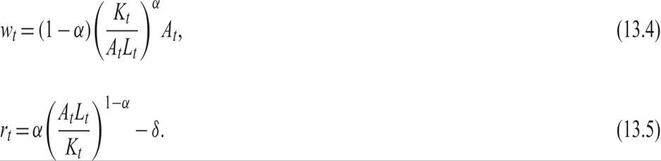
Equations (13.1)–(13.5) describe the behavior of firms. Firms are assumed to employ workers up to the point where the marginal product of labor is equal to the real wage, and capital up to the point where the marginal product of capital equals the real user cost of capital, assumed to be equal to the real interest rate plus the depreciation rate.

13.1.3 The Representative Household

The economy is inhabited by a large number of identical households, each of which has an infinite time horizon. The representative household maximizes its expected intertemporal utility function, which depends on the path of real consumption of goods and services and leisure. The expected intertemporal utility function is defined by

where E is the mathematical expectations operator, and u is the per capita instantaneous utility of the representative household. Per capita consumption is given by c = C/N and per capita employment by l = L/N. Assume that the instantaneous utility function is logarithmic:

where b > 0.

13.1.4 Exogenous Population Growth, Efficiency of Labor, and Government Expenditure

Population increases exogenously at a rate n per period. Consequently,

where 0 < n < ρ.

The final assumptions of the model concern the behavior of the two main exogenous variables. Both productivity (labor efficiency), and government expenditure are supposed to be exogenous stochastic processes.

The stochastic process describing the evolution of the efficiency of labor is given by³

where

It is assumed that − 1 < η_A < 1, and that ε^A is a white noise process. With these assumptions, a_t is a stationary AR(1) process. Equations (13.9) and (13.10) imply that labor efficiency grows at an exogenous rate g, but that it is subject to random disturbances a_t, which follow a stationary first-order autoregressive process. The assumptions about (13.10) imply that the impact of a technological disturbance is gradually reduced over time.

Similar assumptions are made regarding the stochastic process that describes the evolution of real government expenditure. Assume that real government expenditure is growing at an average rate n + g (i.e., on average, it remains constant relative to total output). However, we also assume that real government expenditure is subject to disturbances that follow a stationary first-order autoregressive process. More particularly, assume that

where

It is assumed that − 1 < η_G < 1, and that ε^G is a white noise process. With these assumptions, is a stationary AR(1) process.⁴

These elements complete the structure of the stochastic growth model.

Before we look at the general properties of the model, it is worth considering the implications for the behavior of the representative household of the introduction of leisure in the utility function, as well as the implications of uncertainty in the form of random disturbances.

13.1.5 Labor Supply of the Representative Household

The first difference of this model from the Ramsey model arises from the introduction of leisure time in the utility function of the household, which makes labor supply endogenous. To analyze the importance of this extension, which was first introduced in chapter 2, let us first consider the problem of a household that lives for a single time period and has no assets. The problem of that household is defined as the maximization of

under the constraint

The Lagrange function is defined by

where λ is the relevant Lagrange multiplier. The first-order conditions for a maximum imply that

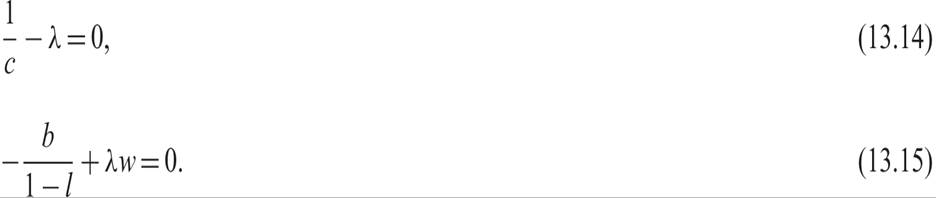
From the budget constraint c = wl and from (13.14), it follows that λ = 1/(wl). Substituting in (13.15), we get

From (13.16), it is apparent that labor supply is independent of the real wage.

However, this inelasticity does not mean that temporary changes in real wages do not affect labor supply even in this case. This can be seen if we look at the behavior of a household that lives for two periods, as assumed in chapter 2.

13.1.6 Intertemporal Substitution in Labor Supply

To see how temporary changes in real wages might affect labor supply (even though with logarithmic preferences, permanent changes in real wages have no effect), let us adopt the simplest intertemporal model, which is none other than the two-period model analyzed in chapter 2. Consider the behavior of a household living for two periods that has no initial wealth and no uncertainty about the real interest rate or the real wage of the second period.

The intertemporal budget constraint of the household is given by

where subscripts 1 and 2 refer to the first and second periods of life, respectively.

The Lagrange function of this household is defined by

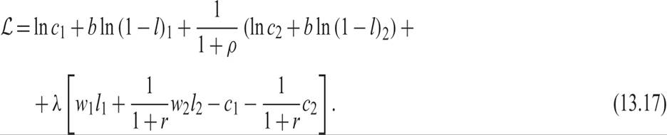
The household chooses consumption and labor supply for each of the two periods. From the first-order conditions for labor supply, we have

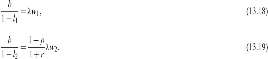
Dividing (13.19) by (13.18) yields

Equation (13.20) implies that the relative labor supply in the two periods depends positively on the relative real wage in the two periods. The higher the real wage of the first period is in relation to that of the second period, the higher will be the labor supply of the first period in relation to that of the second. The household substitutes labor between periods, depending on relative real wages between periods. Because of the assumption of logarithmic preferences, the intertemporal substitution elasticity is equal to one.

Moreover, the higher the real interest rate r is, the greater will be the labor supply of the first period compared to that of the second period. The increase in the interest rate increases the attractiveness of working in the first period and saving for the second period, compared to working in the second period. It has the opposite effect of the pure rate of time preference rate ρ.

These effects of relative wages over time and the real interest rate on labor supply are the intertemporal substitution effects in labor supply that we analyzed in the two-period model of chapter 2. Such effects obviously generalize to a multiperiod setting. Consequently, fluctuations in real wages and the real interest rate can cause fluctuations in employment, even in a model with logarithmic preferences, in which permanent changes in real wages do not affect labor supply.⁵

13.1.7 Uncertainty and the Behavior of the Representative Household

Apart from the endogeneity of labor supply, the second element that differentiates this stochastic growth model from the deterministic Ramsey model is uncertainty arising from the stochastic disturbances. Therefore, the expectations of the representative household for future developments play a significant role.

It is straightforward to show that, for the general case when the household maximizes the expected intertemporal utility function (13.6) subject to the relevant intertemporal budget constraint, the Euler equation for consumption takes the form

The mathematical expectation of the product of two random variables is not equal to the product of their mathematical expectations. It is equal to the product of their mathematical expectations plus the covariance of the two random variables. Thus, (13.21) implies

However, from the first-order conditions for consumption and labor supply, the ratio of consumption to leisure is a positive function of the real wage of the form

Equation (13.23) links labor supply (leisure) and consumption with the real wage. It includes only current variables, as there is no uncertainty in the current period. Equations (13.21) and (13.23) are the two basic equations describing the behavior of households in the stochastic growth model.

We can now examine the properties of the model. This model is not easy to solve analytically, as it contains factors that are both linear and log-linear in the endogenous variables. The properties of the model can be described if we simplify it further, or if we use a log-linear approximation around the balanced growth path and solve it numerically for specific values of the parameters.

In section 13.4, we present the Campbell [1994] log-linear approximation of the full model around its balanced growth path. This allows us to describe the full properties of the model through a numerical simulation around the balanced growth path. However, first let us concentrate on the properties of a simplified version of the model to gain a deeper understanding of its structure.

13.2