Welfare Theorems

We are ultimately interested in equilibrium growth. But in general competitive economies such as those analyzed so far, we know that there should be a close connection between Pareto optima and competitive equilibria.

theorems and develop the relevant connections between the theory of economic growth and dynamic general equilibrium models.

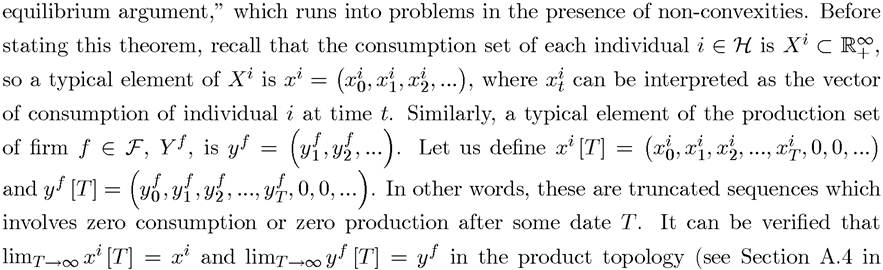
Let us start with models that have a finite number of consumers, so that in terms of the notation above, the setis finite. However, we allow an infinite number of commodities,

since in dynamic growth models, we are ultimately interested in economies that have an

infinite number of time periods, thus an infinite number of commodities. The results stated

in this section have analogs for economies with a continuum of commodities (corresponding to dynamic economies in continuous time), but for the sake of brevity and to reduce technical

of certain commodities. The consumption set is a subset ofsince consumption bundles are represented by infinite sequences and we have imposed the restriction that consumption levels cannot be negative (this can be extended by allowing some components of the vector, corresponding to different types of labor supply, to be negative; this is straightforward and I

book can be done in terms of aggregate production sets.

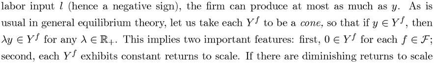
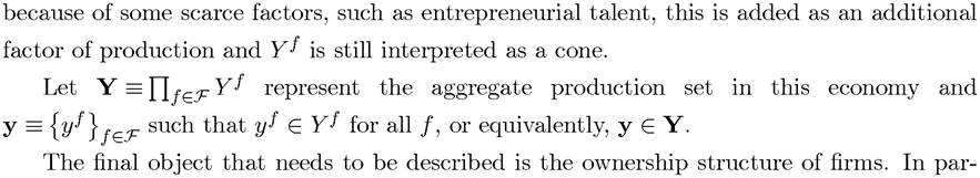
general equilibrium theory, let us assume that there is a finite number of firms represented by the set F and that each firm f ∈ F is characterized by a production set Y^f, which specifies what levels of output firm f can produce from specified levels of inputs. In other words,

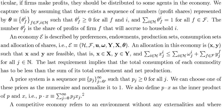
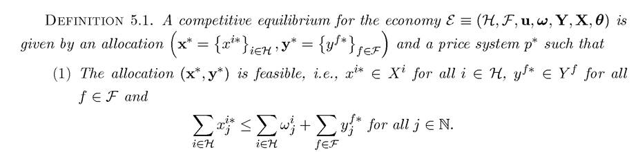
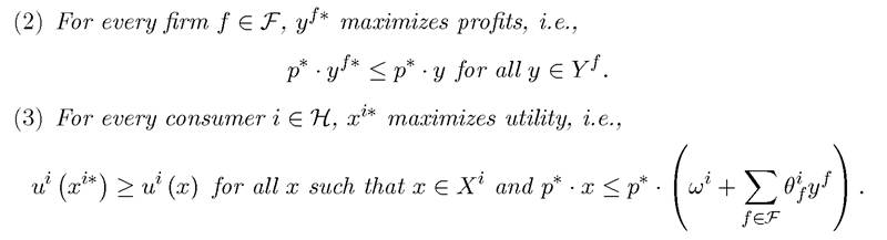
all commodities are traded competitively. In a competitive equilibrium, all firms maximize

profits, all consumers maximize their utility given their budget set and all markets clear. More formally:

₂

²You may note that such an inner product may not always exist in infinite dimensional spaces. But this technical detail does not concern us here, since whenever p corresponds to equilibrium prices, this inner product representation will exist.

A major focus of general equilibrium theory is to establish the existence of a competitive equilibrium under reasonable assumptions. When there is a finite number of commodities and standard convexity assumptions are made on preferences and production sets, this is straight­forward (in particular, the proof of existence involves simple applications of Theorems A.13, A.14, and A.16 in Appendix Chapter A). When there is an infinite number of commodities, as in infinite-horizon growth models, proving the existence of a competitive equilibrium is somewhat more difficult and requires more sophisticated arguments.

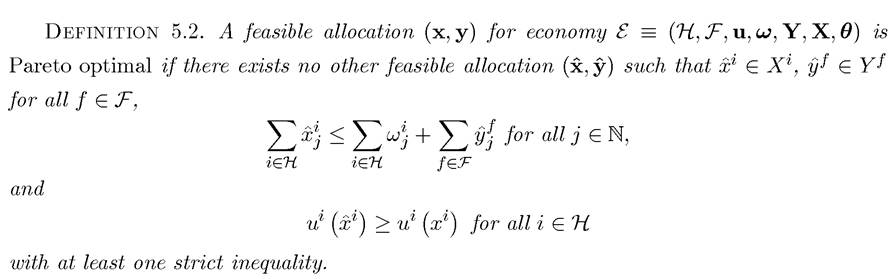
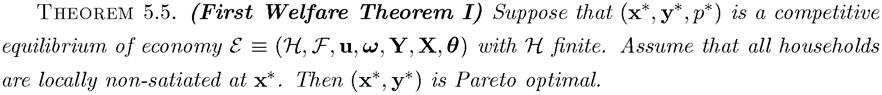
Our next result is the celebrated First Welfare Theorem for competitive economies. Before presenting this result, we need the following definition.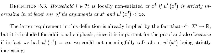

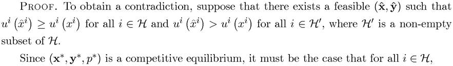
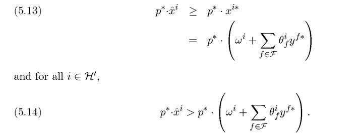
The second inequality follows immediately in view of the fact thatis the utility maximizing choice for household i, thus if x^l is strictly preferred, then it cannot be in the budget set. The first inequality follows with a similar reasoning. Suppose that it did not hold. Then by the hypothesis of local-satiation, u^l must be strictly increasing in at least one of its arguments, let us say the j⁰th component of x. Then constructsuch that is in household i’s budget set and yields strictly greater utility than the original consumption bundle xⁱ, contradicting the hypothesis that household i was maximizing utility.

Also note that local non-satiation implies thatand thus the right-hand sides

of (5.13) and (5.14) are finite (otherwise, the income of household i would be infinite, and the household would either reach a point of satiation or infinite utility, contradicting the local non-satiation hypothesis).

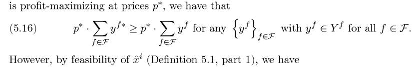
Now summing over (5.13) and (5.14), we have

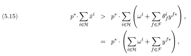
where the second line uses the fact that the summations are finite, so that we can change the order of summation, and that by definition of shares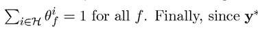

The proof of the First Welfare Theorem is both intuitive and simple. The proof is based on two intuitive ideas. First, if another allocation Pareto dominates the competitive equilibrium, then it must be non-affordable in the competitive equilibrium. Second, profit­maximization implies that any competitive equilibrium already contains the maximal set of affordable allocations. It is also simple since it only uses the summation of the values of commodities at a given price vector. In particular, it makes no convexity assumption. However, the proof also highlights the importance of the feature that the relevant sums exist and are finite. Otherwise, the last step would lead to the conclusion thatwhich

may or may not be a contradiction. The fact that these sums exist, in turn, followed from two assumptions: finiteness of the number of individuals and non-satiation. However, as noted before, working with economies that have only a finite number of households is not always sufficient for our purposes.

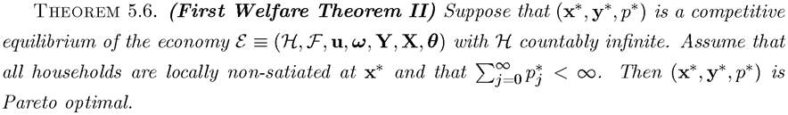
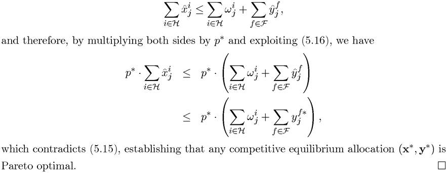
Proof. The proof is the same as that of Theorem 5.5, with a major difference. Local non-satiation does not guarantee that the summations are finite (5.15), since we have the sum 198

over an infinite number of households. However, since endowments are finite, the assumption thatensures that the sums in (5.15) are indeed finite and the rest of the proof

goes through exactly as in the proof of Theorem 5.5. ?

Theorem 5.6 will be particularly useful when we discuss overlapping generation models.

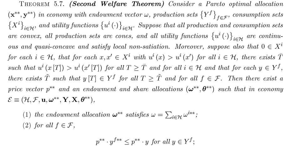
We next briefly discuss the Second Welfare Theorem, which is the converse of the First Welfare Theorem. It answers the question of whether a Pareto optimal allocation can be decentralized asa competitive equilibrium. Interestingly, for the Second Welfare Theorem whether or notis finite is not as important as for the First Welfare Theorem. Nevertheless,

the Second Welfare Theorem requires a number of assumptions on preferences and technology,

such as the convexity of consumption and production sets and preferences, and a number of additional requirements (which are trivially satisfied when the number of commodities is finite). This is because the Second Welfare Theorem implicitly contains an “existence of

Appendix Chapter A).

I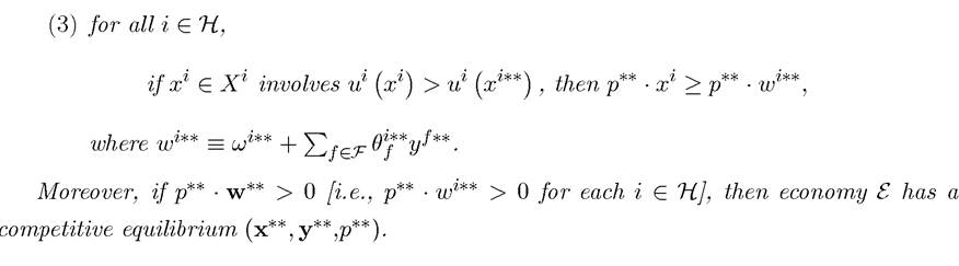

The proof of this theorem involves the application of the Geometric Hahn-Banach Theo­rem, Theorem A.25, from Appendix Chapter A. It is somewhat long and involved. For this reason, a sketch of this proof as provided in the next (starred) section. Here notice that if instead of an infinite-dimensional economy, we were dealing with an economy with a finite commodity space, say with K commodities, then the hypothesis in the theorem, that 0 ∈ Xⁱ 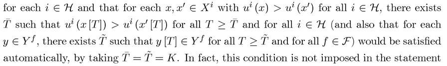of the Second Welfare Theorem in economies with a finite number of commodities. Its role in dynamic economies, with which we are concerned with in this book, is that changes in allocations that are very far in the future should not have a “large” effect on preferences. This is naturally satisfied when we look at infinite-horizon economies with discounted utility and separable production structure. Intuitively, if a sequence of consumption levels x is strictly preferred to x⁰, then setting the elements ofto 0 in the very far (and thus heavily discounted) future should not change this conclusion (since discounting implies that x could not be strictly preferred to x⁰ because of higher consumption under x in the arbitrarily far future). Similarly, if some production vector y is feasible, the separable production structure implies that y [T], which involves zero production after some date T, must also be feasible. Exercise 5.13 demonstrates these claims more formally. One difficulty in applying this theo­rem is that uⁱ may not be defined when x has zero elements (so that the consumption set Xⁱ does not contain 0). Exercise 5.14 shows that the theorem can be generalized to the case in which there exists a strictly positive vectorwith each element sufficiently small and with

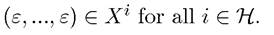
The conditions for the Second Welfare Theorem are more difficult to satisfy than those for the First Welfare Theorem because of the convexity requirements. In many ways, it is also the more important of the two theorems. While the First Welfare Theorem is celebrated as a formalization of Adam Smith’s invisible hand, the Second Welfare Theorem establishes the stronger results that any Pareto optimal allocation can be decentralized as a competitive equilibrium. An immediate corollary of this is an existence result; since the Pareto optimal 200

allocation can be decentralized as a competitive equilibrium, a competitive equilibrium must exist (at least for the endowments leading to Pareto optimal allocations).

The Second Welfare Theorem motivates many macroeconomists to look for the set of Pareto optimal allocations instead of explicitly characterizing competitive equilibria. This is especially useful in dynamic models where sometimes competitive equilibria can be quite difficult to characterize or even to specify, while social welfare maximizing allocations are more straightforward.

The real power of the Second Welfare Theorem in dynamic macro models comes when we combine it with models that admit a representative household. Recall that Theorem 5.3 shows an equivalence between Pareto optimal allocations and optimal allocations for the representative household. In certain models, including many—but not all—growth models studied in this book, the combination of a representative household and the Second Welfare Theorem enables us to characterize the optimal growth allocation that maximizes the utility of the representative household and assert that this will correspond to a competitive equilibrium.

5.7.