Article 13.2 Investors bet on junk bonds to outperform
By Vivianne Rodrigues and Michael Mackenzie
Financial Times July 30, 2013
The average junk yield, which moves inversely to prices, has dipped below 6% this month, a big turnround in sentiment when the 10-year Treasury yield of 2.60% remains just shy of its June peak.
The total return for an index of US junk bonds in July stands at 2%, according to Barclays. Year-to-date, high yield has returned 3.4%. While investment-grade bonds have rallied 1% in July, the sector has posted a negative 2.4% total return for the year. The contrast in performance between junk and investment grade reflects a stark difference in the sensitivity of bonds in an environment of rising interest rates.
Investment-grade bonds tend to carry lower coupons over longer maturities, which in turn helps increase the bonds' so-called duration - a measure of how sensitive bond prices are to changes in interest rates.
For example the average duration for junk debt stands at 4.2 years, below the average of 6.9 years for investment-grade bonds for the respective Barclays bond indices that are followed by money managers.
The lower a bond's duration, the less its price reacts to change in underlying interest rates.
Source: Rodrigues, V. and Mackenzie, M. (2013) Investors bet on junk bonds to outperform, Financial Times, 30 July.
Duration if coupons increase
If we take two bonds with the same yield to maturity, but one has higher coupons, then duration will be lower on that bond, resulting in a bond with less volatility or interest rate risk. To illustrate we can go back to the example of the four-year bond above with a yield to maturity of 7% (Table 13.3). We can compare its duration with that for another bond with the same yield to maturity but with the following pattern of cash flows:
Current market price = £144.03
Four annual coupons of £20
Par (nominal) value to be redeemed in four years = £100
Table 13.5 Calculating duration on a four-year 20% coupon bond when the yield to maturity remains at 7%
| Period | Coupon and principal | PV (7% discount rate, the current market YTM) | Weights (PV ÷ total PV as a percentage) | Weighted maturity value (period ? weights ÷ 100) in years | ||
| 1 | £20 | £18.69 | (£18.69 ÷ £144.03) ? 100 = | 12.98% | 1 ? 12.98 ÷ 100 = | 0.1298 |
| 2 | £20 | £17.47 | (£17.47 ÷ £144.03) ? 100 = | 12.13% | 2 ? 12.13 ÷ 100 = | 0.2426 |
| 3 | £20 | £16.32 | (£16.32 ÷ £144.03) ? 100 = | 11.33% | 3 ? 11.33 ÷ 100 = | 0.3399 |
| 4 | £120 | £91.55 | (£91.55 ÷ £144.03) ? 100 = | 63.56% | 4 ? 63.56 ÷ 100 = | 2.5424 |
| Total PV | £144.03 | 100.00% | Duration = | 3.2547 years | ||
The bond with £20 coupons has a shorter duration, at 3.2547 years, than the bond with the £7 coupon, at 3.6243 years, despite the yield to maturity and time to maturity remaining the same.
Thus we come to another rule:The higher the coupon rate on the bond, the shorter the bond's duration.
Using duration as a guide to interest rate risk
As duration increases, the percentage change in the market value of a bond increases for a given change in interest rates, i.e. interest rate risk rises with duration. Thus we can use duration as a measure of interest rate risk. It is not a perfect measure, but it does provide a good approximation, when interest rate changes are small, of the extent to which the price of a bond will change if yields to maturity rise or fall - as expressed in the following formula:
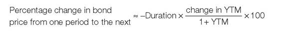
The negative sign in front of Duration is due to the inverse relationship between bond prices and interest rates.
For example, if an investor is holding the four-year bond yielding 7% at time t in Table 10.3 with a duration of 3.6243 years, you could ask: how much would the price of the bond change if interest rates (YTM) rose by 1%?
Answer:
Change in interest rate = 0.01
Current YTM = 0.07

Thus, for a 1 percentage point change in market interest rates this bond's price moves by roughly 3.39%. (Note that this formula can only be used for small changes in yield to maturity of one percentage point or less, and even then it is only an approximation. It slightly overestimates price declines and underestimates price increases - see convexity discussion later.) We can compare this degree of sensitivity to interest rate changes with other bonds. Let us take the four-year bond in Table 13.5 offering 20% coupons with YTM of 7%. It has a duration of 3.2547 years.

Clearly, this bond carries less interest rate risk than the 7% coupon bond, as its price changes by only 3.04% when yields change by 1 percentage point.
The lower duration and therefore lower interest rate risk, but same yield to maturity, on the 20% coupon bond may induce an investor to switch investment funds from the more risky bond (7% coupon) to this less risky one.Convexity
In the section discussing the effect of duration on interest rate risk we noted that the formula, while roughly correct, produces errors for the influence of interest rate changes on bond pricing. This is because it assumes a linear relationship between interest rate changes and bond price changes - this is shown by the straight diagonal line in Figure 13.1. The exact valuation relationship is curved, and the curvature around some interest rate level is measured by convexity. The true relationship line is tangential to the straight line assumption only at a zero interest rate change, i.e. it has the same slope, therefore for very small interest rate changes the duration approach gives the true answer. However, if we test large interest movements the true bond price changes are different to that determined by the duration-based calculation we used earlier.
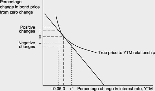
Figure 13.1 The linear assumption for the relationship between bond price and YTM
This can be illustrated using the same example above, where we calculated a change in bond price of -3.39% for a 1% increase in yield to maturity. We can now calculate the actual change for an increase in 1%. At the interest rate of 7% the four-year bond was priced at £100. If interest rates rise to 8% then the price changes to £96.6877:
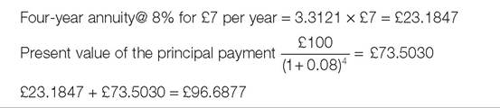
This is a -3.3123% change ((100 - 96.6877) ÷ 100), a true percentage change resulting from the rise in YTM. Compare this with the approximation provided by using a duration of -3.39%. When interest rates rise, the true decline in price is less than the fall implied using duration.
Bond market participants often want to use duration to estimate sensitivity of price to YTM changes. This can be done more accurately if they allow for the extent of convexity. More precisely, they need to measure the curve at that particular interest rate because slopes alter with the starting point for YTM changes. This involves formidable calculations which are beyond the scope of this book. Bond traders do not always need to carry out these calculations to make decisions because they develop an ability to gain a ‘good enough' idea of
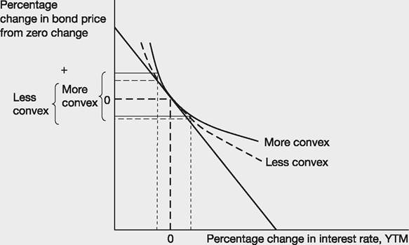
Figure 13.2 High convexity versus low convexity
bond price changes given the maturity and coupon rate to form a view of the ball-park movements in various scenarios. Besides, modern computer systems calculate duration and convexity automatically and display them on trading screens.
For bond investors, high convexity is usually a desirable quality and so they pay premiums to hold such bonds. This can be understood by examining Figure 13.2. Two bonds are shown, each with the same duration at point ‘0' (no change in interest rate), but one has greater convexity. If interest rates increase, the one with the greater convexity will experience a lower percentage decrease in price than the bond with lower convexity. However, if rates decline, the high convexity bond will have a greater uplift in value than the low convexity bond.
The term structure of interest rates
It is not safe to assume that the yield to maturity on a bond will remain the same regardless of the length of time of the loan (holding all else constant). So, if the interest rate on a three-year bond is 7% per year, it may or may not be 7% on a five-year bond of the same risk class and liquidity class. Lenders in the financial markets demand different interest rates on loans of differing lengths of time to maturity - that is, there is a term structure of the interest rates.
Four of these relationships are shown in Figure 13.3 for lending to the UK, US,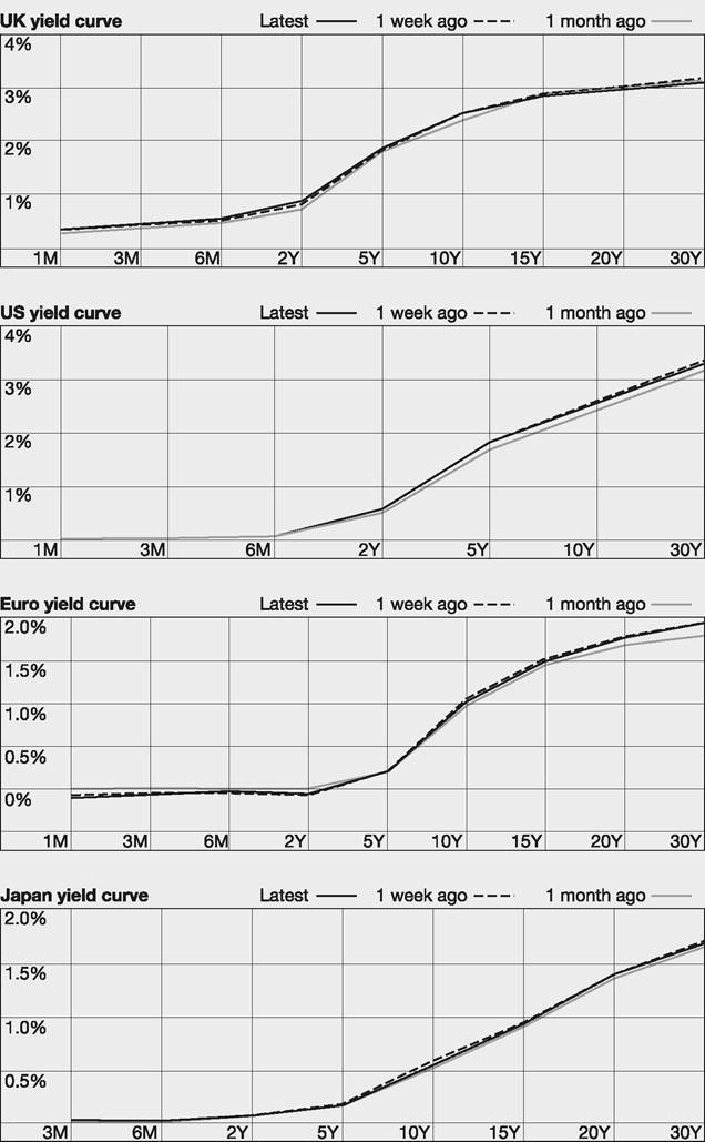
Figure 13.3 Yield curves for the UK, US, eurozone and Japanese government bills and bonds (The ‘Latest' shows the current rates for different maturities. Also shown is the range of rates as calculated one week before and one month before)
Source: The Financial Times
eurozone andJapanese governments.[30] Note that default (and liquidity) risk remains constant along one of the lines; the reason for the different rates is the time to maturity of the bonds. Thus, a two-year US government bond has to offer 0.57% whereas a ten-year bond offered by the same borrower gives 2.62%. Note that the yield curve for the eurozone is only for the most creditworthy governments who have adopted the euro (e.g. Germany). Less safe governments had to pay a lot more in 2014 as investors worried whether they would default.
Upward-sloping yield curves occur in most years, but 2014 demonstrated extreme upward slopes because governments and central banks around the world forced down short-term interest rates. Occasionally we have a situation where short-term interest rates (lending for, say, one year) exceed those of long-term interest rates (say, a 20-year bond). A downward-sloping term structure (yield curve inversion), a flat yield curve and the usual upward-sloping yield curves are shown in Figure 13.4.
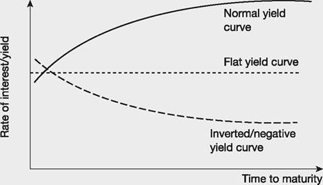
Figure 13.4 Upward-sloping, downward-sloping and flat yield curves
Three main hypotheses have been advanced to explain the shape of the yield curve (these are not mutually exclusive - all three can operate at the same time to influence the curve):
a The expectations hypothesis.
b The liquidity-preference hypothesis.
c The market-segmentation hypothesis.
The expectations hypothesis
The expectations hypothesis focuses on the changes in interest rates over time.
To understand the expectations hypothesis you need to know what is meant by a spot rate of interest. The spot rate is an interest rate fixed today on a loan that is made today. So a corporation, Hype plc, might issue one-year bonds at a spot rate of, say, 8%, two-year bonds at a spot rate of 8.995% and three-year bonds at a spot rate of 9.5%. This yield curve for Hype is shown in Figure 13.5. The interest rates payable by Hype are bound to be greater than for the UK government across the yield curve because of the additional default risk on these corporate bonds compared with safe government bonds.Spot rates change over time. The market may have allowed Hype to issue one-year bonds yielding 8% at a point in time in 2014 but a year later (time 2015) the one-year spot rate may have changed to become 10%. If investors expect that one-year spot rates will become 10% at time 2015 they will have a theoretical limit on the yield that they require from a two-year bond when
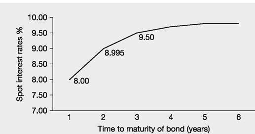
Figure 13.5 The term structure of interest rates for Hype plc at time 2014
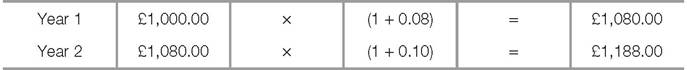
viewed from time 2014. Imagine that an investor (lender) wishes to lend £1,000 for a two-year period and is contemplating two alternative approaches:
1 Buy a one-year bond at a spot rate of 8%; after one year has passed the bond will come to maturity. The released funds can then be invested in another one-year bond at a spot rate of 10%, expected to be the going rate for bonds of this risk class at time 2015.5
2 Buy a two-year bond at the spot rate at time 2014.
Under the first option the lender will have a sum of £1,188 at the end of two
years:
Given the anticipated change in one-year spot rates to 10% the investor will buy the two-year bond only if it gives the same average annual yield over two years as a series of one-year bonds (the first option). The annual interest required will be:
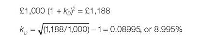
which is the spot rate quoted for a two-year bond in 2014 in the second option.
Thus, it is the expectation of spot interest rates changing that determines the shape of the yield curve according to the expectations hypothesis.
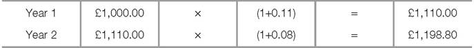
Now consider a downward-sloping yield curve where the spot rate on a one- year instrument is 11% and the expectation is that one year from now spot rates will fall to 8% for the one-year bonds. An investor considering a two-year investment will obtain an annual yield (k) of 9.49% by investing in a series of one-year bonds, viz:
[1] I have simplified this to spot rates only. In reality investors in bonds can agree to buy a bond one year (or more years) from now, a forward. The price of the forward purchase is agreed now, thus traders can lock in the interest rate from that point on. This implied forward rate can be interpreted as the market's consensus of the spot rates in one year from now.
or £1,000 (1.11) (1.08) = £1198.80
With this expectation for movements in one-year spot rates, lenders will demand an annual rate of return of 9.49% from two-year bonds of the same risk class.
Thus in circumstances where short-term spot interest rates are expected to fall, the yield curve will be downward sloping.
Example 13.7
Spot rates
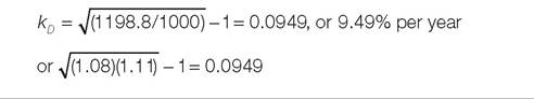
If the present spot rate for a one-year bond is 5% and for a two-year bond is 6.5%, what is the expected one-year spot rate in a year's time?
Answer
If the two-year rate is set to equal the rate on a series of one-year spot rates then: 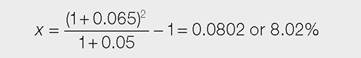
The liquidity-preference hypothesis
The expectations hypothesis does not adequately explain why the most common shape of the yield curve is upward sloping. The liquidity-preference hypothesis (liquidity premium theory) helps explain the upward slope by pointing out that investors require an extra return for lending on a long-term basis. Lenders demand a premium return on long-term bonds compared with short-term instruments because of greater interest rate risk and the risk of misjudging future interest rates. Putting your money into a ten-year bond on the anticipation of particular levels of interest rates exposes you to the possibility that rates will rise above the rate offered on the bond at some point in its long life. Thus, if five years later interest rates double, say because of a rise in inflation expectations, the market price of the bond will fall substantially, leaving the holder with a large capital loss if they sell. By investing in a series of one-year bonds, however, the investor can take advantage of rising interest rates as they occur. The ten-year bond locks in a fixed rate for the full ten years if held to maturity. Investors prefer short-term bonds so that they can benefit from rising rates and so will accept a lower return on short-dated instruments.
The liquidity-preference theory focuses on a different type of risk attaching to long-dated debt instruments other than default risk - a risk related to uncertainty over future interest rates. A suggested reinforcing factor to the upward slope is that borrowers usually prefer long-term debt because of the fear of having to repay short-term debt at inopportune moments. Thus borrowers increase the supply of long-term debt instruments, adding to the tendency for long-term rates to be higher than short-term rates.
A further factor is that in many bond markets there is a greater volume of trading for short-dated instruments than longer-dated ones, i.e. there is greater liquidity, an increased speed and ease of the sale of an asset. In bond markets where there is high liquidity for both short- and long-term bonds, the title ‘liquidity-preference theory' seems incorrectly used because there is no problem of illiquidity for long-term bonds. For example, for government bonds, sale in the secondary market is often as quick and easy as for short-term bonds. In the bond markets where liquidity is fairly constant along the yield curve, the premium for long-term bonds is generally compensation for the extra risk of capital loss; ‘term premium' might be a better title for the hypothesis.
The market-segmentation hypothesis
The market-segmentation hypothesis argues that the debt market is not one homogeneous whole but that there are, in fact, a number of sub-markets defined by maturity range. The yield curve is therefore created (or at least influenced) by the supply and demand conditions in each of these sub-markets. For example, banks tend to be active in the short-term end of the market and pension funds to be buyers in the long-dated segment.
If banks need to borrow large quantities quickly they will sell some of their short-term instruments, increasing the supply on the market, so pushing down the price and raising the yield. Meanwhile, pension funds may be flush with cash and may buy large quantities of 20-year bonds, helping to temporarily move yields downward at the long end of the market. At other times banks, pension funds and the buying and selling pressures of a multitude of other financial institutions will influence the supply and demand position in the opposite direction. The point is that the players in the different parts of the yield curve tend to be different. This hypothesis helps to explain the often lumpy or humped yield curve.
A final thought on the term structure of interest rates
It is sometimes believed that in circumstances of a steeply rising yield curve it would be advantageous to borrow short term rather than long term. However, this can be a dangerous strategy because long-term debt may be trading at a higher rate of interest because of the expected rise in spot short-term rates and so when the borrower comes to refinance in, say, a year's time, the short-term interest rate is much higher than the long-term rate and this high rate has to be paid out of the second year's cash flows, which may not be convenient.
Additional reading
Bodie, Z., Kane, A. and Marcus, A.J. (2014) Investments. McGraw-Hill.
Chisholm, A.M. (2009) An Introduction to International Capital Markets. 2nd edition. John Wiley & Sons.
Choudry, M. (2010) An Introduction to Bond Markets. 4th edition. John Wiley & Sons.
Fabozzi, F.J. (2012) Bond Markets, Analysis and Strategies. 8th edition. Prentice Hall.
Veronesi, P. (2010) Fixed Income Securities. John Wiley & Sons.