[88] Silver Shocks and Stock Price Movements
The Granger-causality effects discussed earlier remain limited to the effects of silver prices on nominal variables, owing to the absence of usable series on real variables like output. Although annual estimates by Yeh (1979, p. 97) do suggest that an 8.7% drop in China’s real GDP accompanied the
Table 5.6.
Granger-Causality Tests on inflation, the exchange rate, and silver prices | Causal Relationship Tested | F-Statistic |
1928:01 -1935:10
| US Silver Price → Inflation | 3.27** [0.0152] |
| Inflation → US Silver Price | 0.87 [0.4854] |
| Exchange Rate → Inflation | 7.23*** [0.0000] |
| Inflation → Exchange Rate | 0.81 [0.5241] |
| Exchange Rate → US Silver Price | 4.55*** [0.0022] |
| US Silver Price → Exchange Rate | 1.43 [0.2323] |
1928:01 -1937:06
| US Silver Price → Inflation | 1.79 [0.1356] |
| Inflation → US Silver Price | 0.88 [0.4770] |
| Exchange Rate → Inflation | 10.14*** [0.0000] |
bgcolor=white>Inflation → Exchange Rate | 0.62 [0.6507] |
| Exchange Rate → US Silver Price | 5.21*** [0.0007] |
| US Silver Price → Exchange Rate | 1.11 [0.3568] |
Notes: ***, **, and * denote significance at the 99%, 95%, and 90% levels, respectively; the figures in brackets are the exact significance levels (P-values); and four lags have been included in each of the test regressions.
onset of US silver purchases in 1934, Brandt and Sargent (1989) and Rawski (1989, 1993) point to Chinese banks’ ability to expand their note issues sufficiently to offset the decline in silver money as world silver prices rose - thereby helping limit (or, much more arguably, eliminate) the negative deflationary effects discerned by Friedman (1992) and many contemporary accounts (see also Burdekin, 2008).
In the absence of reliable and consistent data on Chinese real economic performance, monthly stock market data offer an alternative, relatively high-frequency window that could shed light on the real effects of silver price movements. Table 5.7. Granger-Causality with the real silver price in the three-equation system
| Causal Relationship Tested | F-Statistic |
1928:01 -1935:09
| US Silver Price → Inflation | 3.00** [0.0229] |
| Inflation → US Silver Price | 0.57 [0.6819] |
| Exchange Rate → Inflation | 7.23*** [0.0000] |
| Inflation → Exchange Rate | 0.81 [0.5241] |
| Exchange Rate → US Silver Price | 3.45** [0.0116] |
| US Silver Price → Exchange Rate | 0.80 [0.5266] |
1928:01 -1937:06
| US Silver Price → Inflation | 1.97 [0.1047] |
| Inflation → US Silver Price | 1.26 [0.2911] |
| Exchange Rate → Inflation | 1014*** [0.0000] |
| Inflation → Exchange Rate | 0.62 [0.6507] |
| Exchange Rate → US Silver Price | 3.61*** [0.0085] |
| US Silver Price → Exchange Rate | 0.65 [0.6253] |
Notes: ***, **, and * denote significance at the 99%, 95%, and 90% levels, respectively; the figures in brackets are the exact significance levels (P-values); and four lags have been included in each of the test regressions.
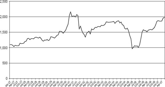
This section focuses on the evolution of the HSBC stock price over the 1927-1937 period, thereby taking advantage of a consistent data series on an institution that stood out as a major player in both Chinese and Hong Kong financial markets. HSBC actually operated as an official arm of Chinese monetary policy prior to the Nanking decade and remained “the most important foreign bank in China [that] had long dominated international financethere... ’’(Schenk,2002). HSBChas,ofcourse,retaineditsposition as a major international bank to this day. HSBC stock traded actively in London and Shanghai as well as in Hong Kong. Although the data employed
![]()
Figure 5.5. Hongkong and Shanghai Banking Corporation, January 1927-June 1937 (month-end closing share price in Hong Kong).
in this section are taken from the Hong Kong market, stock prices were generally very similar across markets, reflecting the availability of telegraph communications (Bailey and Bhaopichitr, 2004, p. 146). The HSBC data series spans the period both before and after China’s monetary reform on November 5,1935 that freed the note issue from its old link to the shrinking stock of available silver.[89]
HSBC’s trading price over the January 1927 to June 1937 period is plotted in Figure 5.5, revealing sustained gains over the late 1920s followed by sharp declines in 1931 and 1934-1935. These declines themselves appear to coincide, first, with the British and Japanese break from gold - coupled with the September 1931 Japanese invasion of Manchuria - and, second, with the sharp rise in silver prices following the implementation of the US silver purchase program. Econometric analysis confirms that each of these declines represented a nonreversed “turning point” in the equity series. The HSBC stock price is initially simply modeled as a function of its own past history, with such series often displaying a certain degree of inertia whereby past movements, on average, help predict future movements.
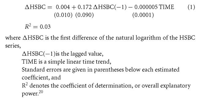
After converting the stock price series into log first difference form to assure stationarity, allowance was made for effects of lagged values going back four months together with a constant and a time trend. Only one lag, that is the prior month’s value, was found to be significant, leading to the following basic specification: ![]()
The results suggest that the effect of the lagged stock price change is positive and significant at the 94% confidence level. Although the overall explanatory power of the basic equation is low, the next step is to allow for additional dummy variables that can capture possible shifts in the equation over the sample period and, hence, better explain the major ups and downs. Following the general procedure suggested by Banerjee, Lumsdaine, and Stock (1992), the data were organized into a series of non-overlapping “windows,” each being a year in length. Repeated estimation, progressively moving through the overall sample period, reveals those windows, or portions of the sample, where especially low R2 values make the presence of a structural break most likely. Dummy variables are then defined successively for each week in the period surrounding the window in question, with these dummies taking on a value of one for that week and every week thereafter. The week for which this “rolling” estimation procedure yields the highest dummy variable significance level then forms our best estimate of the exact date at which a nonreversed “turning point” occurs.[90] [91] The most significant breakpoints for the HSBC series are presented in Table 5.8. The results suggest that negative turning points in the series occurred in March and September 1931. The latter downturn occurs in the same month as the United Kingdom’s exit from the gold standard andJapan’s
Table 5.8. Potential TurningPoints in the Hong Kong and Shanghai Bank Corporation Stock Price Series
| Date | t-Statistic |
| March 1931 | -2.557*** |
| September 1931 | -2.151** |
| February 1932 | 2.055** |
| March 1932 | 3.922*** |
| June 1934 | -2.622*** |
| August 1934 | -2.061** |
| May 1935 | 1.849* |
Notes: The t-statistics reflect the sign and significance of the coefficient attached to a dummy variable defined for the month in question, and **7*, and * denote significance at the 99%, 95%, and 90% confidence levels, respectively.
invasion of Manchuria. The UK policy action gave rise to depreciation of the pound against the Chinese currency whereas the loss of Manchuria deprived China of a key source of industrial production and 15% of its overall customs revenues (Young, 1971, p. 200). The earlier turning point indicated for March 1931 appears to coincide with a correction from the sharp share price advance that began during the summer of 1930, but is not obviously tied to major historical events. Meanwhile, the positive turning point suggested for March 1932 saw HSBC’s stock price begin a partial recovery from the steep downturn initiated in September 1931. The gains continued until 1934 and perhaps reflect the fact that business conditions in Shanghai were not, at first, so adversely affected by the 1931 events, with inflows of silver from China’s interior more than compensating for the outflow abroad (as discussed earlier).
Successive negative turning points are indicated for June 1934 and August 1934. The first negative turning point coincides with the passage of the US Silver Purchase Act on June 19, 1934. Although large-scale purchases did not get underway until the following month, the act clearly presaged new upward pressure on silver prices and hence additional upward pressures on China’s currency. Meanwhile, August 1934 stands out as the month with the most dramatic increase in the silver drain prior to China’s November 1935 break from silver (see Table 5.4). BothJune 1934 and August 1934 were therefore months that contained plenty of bad news for business interests in Shanghai and for the silver-standard economies generally. The specific dates of the negative turning points appear to point, rather unambiguously, to a negative reaction to the initiation, and effects, of the US Silver Purchase Act. HSBC’s stock price certainly dropped precipitously after the act was passed, falling by over 46% between June 1934 and April 1935 - at the very least suggesting that the act was not favorably received by the bank’s investors.
After bottoming out in April 1935, HSBC’s stock price enjoyed a limited “bounce” followed by accelerating gains after the November 1935 currency reform. HSBC’s share price rose by just under 13% between April and October 1935 before embarking on a near 82% advance between October 1935 and June 1937. The significant positive turning point identified for May 1935 coincides with the initial recovery from the low recorded in April 1935 but precedes the larger advance that, based on the raw data displayed in Figure 5.5, appeared to correspond with the November 1935 break from silver. The turning point procedure is, unfortunately, often unable to distinguish breaks in nearby months, and identification is further hampered when proximity to the end of the sample leaves little time for the turning point to be established in the data. The bottom line is that we see evidence that the stock price recovered in 1935, even though the empirical procedure cannot precisely tie the recovery to the actual month of the currency reform.
Overall, the turning point analysis, first, offers empirical confirmation of the negative effects generally attributed to the United Kingdom’s exit from the gold standard and the Japanese invasion of Manchuria. Following partial recovery in 1932, renewed successive negative turning points arise just when the US Silver Purchase Act was passed and large-scale silver purchases began. HSBC’s stock plunged after these latter events, and, although there is evidence of a positive turning point as early as May 1935, large gains were postponed until after China’s break from silver later in the year.