The Classical Theory of Economic Policy with Fixed and Flexible Targets
This section largely draws on Acocella, Di Bartolomeo and Hughes Hallett (2013: chap. 2).
1.6.1 TheFixed-TargetApproach
The static economic relationships between variables are defined by the following general linear algebraic system:

where y∈Rq is the vector of relevant economic variables (the government’s target variables) whose generic entry is denoted by ó(i), extracted from Y; u∈Rm is the vector of the government’s policy instruments, whose generic element is denoted by č(j), extracted from Z; A and B are appropriately parameterised target and instrument coefficient matrices, and k is an appropriate vector of constants, each component of which is a linear combination of constants, exogenous variables and white-noise shocks.
We assume - without loss of generality - that A and B are full-rank matrices; i.e. all targets and instrument variables are linearly independent of each other. There are q distinct targets and m distinct instruments to be chosen and set, respectively, by the government.
The linear ‘reduced-form’ model can be derived from (1.1) as follows:

provided that A is nonsingular, as it is from our rank assumptions. Matrix C is a matrix of multipliers and is sometimes called the ‘Jacobian matrix’. Element C(i, j) indicates the effect on target i of changes in instrument j; i.e. ∂y(i)∕∂u(j). Policy effectiveness and policy neutrality can be defined in terms of (1.2).
Policy Effectiveness. An instrument, e.g. instrument č(j), is ineffective with respect to target ó (i) if changes in that instrument determine no changes in the target variable. In this case, C(i, j) = 0.
Otherwise, it is effective.(Exogenous) Policy Neutrality. Economic policy is neutral with respect to a target variable if all the instruments are ineffective with respect to that target variable. In this case, the row entries of matrix C are all zeros.
The aim of the government is to control the economic system (1.2). This will involve finding values of the instruments that enable it to reach any desired values of the target variables y∈Rq (‘target values') in their economy; i.e. the vector u that solves the equation y = Cu can always be found for all possible desired values of y. The system is weakly controllable if a given (specific) vector of target values can be reached. Controllability clearly implies weak controllability, but not conversely. Moreover, it should be noticed that controllability is in fact an existence condition for suitable policy instrument values (‘existence problem'). However, controllability ensures neither the uniqueness of the policy (‘uniqueness problem') nor how best to determine it (‘policy design problem'). Notice also that controllability clearly implies policy non-neutrality, but the converse is not true.
Existence conditions for a solution are easily found by applying standard mathematical techniques. Usually these are rank conditions on certain coefficient matrices or transformations of those matrices.
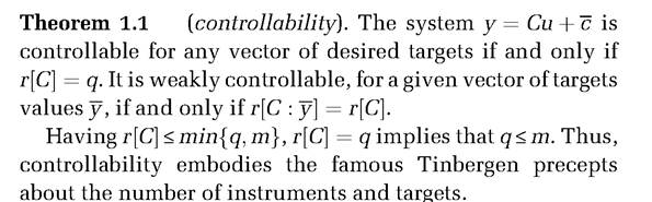
Theorem 1.2 (Tinbergen theorem or static controllabil
ity). The government can achieve any vector of independent targets by an appropriate vector of instruments if and only if the number of independent instruments is equal to or greater than the number of targets.
Formally, the Tinbergen theorem comprises two conditions (Preston and Pagan 1982):
1. A counting rule, according to which the number of instruments should be greater than or equal to the number of targets, i.e. q ≤ m; and
2. An independence rule stating that the (linearly) independent instruments are at least q in number if this is the number of independent targets.
This result must be qualified. In fact, if some of the instruments have value of their own (e.g. as they might imply distortions, causing losses), their number can be lower than that of targets, which include some of the instruments.
Assuming that the policy model fails to satisfy the appropriate weak or strong existence criterion of controllability, the first best policy cannot be achieved. The failure to find a solution for the fixed-target problem in those cases generates the need for some alternative, which we discuss in Section 1.6.2.
1.6.2 The Flexible-Target Approach
The flexible-target approach is based on the minimisation of a ‘loss function'. A useful formalisation of the government's cost for deviations of the relevant variables from their target values is the following quadratic form:
where Q is an appropriate symmetric, positive-definite matrix of relative priorities between the target variables. In (1.4) we do not explicitly consider instrument costs. We refer to y and Q as the parameters of the government’s preferences.
Quadratic functions are used not only for their mathematical tractability but also for their useful economic properties. In fact, deviations from the target in either direction are associated with increasing costs. The marginal rate of substitution between any couple of target variables is therefore never constant but depends on the values of the two variables at the point at which they are computed. In addition, quadratic forms can be obtained as second-order Taylor approximations of more complex functions.
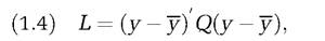
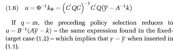
The flexible-target policy is obtained by minimising (1.4) with respect to the vector of instruments, subject to (1.2). The corresponding first-order condition is
The policy design problem therefore implies the following optimal policies:
17
If Q is a positive-definite matrix, then r[C'QC] = r[C] for any conformable matrix C.
When considering the flexible-target approach, any policy is endogenous and depends on the policymaker’s preferences. For this reason, we find it convenient to redefine neutrality as follows.
(Endogenous) Policy Neutrality. Economic policy is neutral with respect to a target variable if the optimal value of such a variable is not affected by any change in the policymaker’s preferences.
This definition generalises that of exogenous neutrality in the same way as the flexible-target approach to policymaking nests the fixed-target approach. In the chapters that follow, we focus on strategic contexts where policies are always endogenous, and when speaking of neutrality, we will always refer to the concept of endogenous policy neutrality instead of the concept of exogenous neutrality.
A geometric representation of the cases of fixed and flexible targets can be useful. We can now give an example of the geometric representation of the problem of fixed targets. Consider an aggregate demand-aggregate supply (AD-AS) representation of the economy, as taken from Hansen (1968) and reproduced by Preston and Pagan (1982): 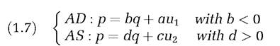
The reduced form of system is
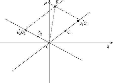
Figure 1.1 Fixed-target approach.
(Source: Acocella, Di Bartolomeo and Hughes Hallett 2013)
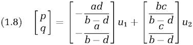
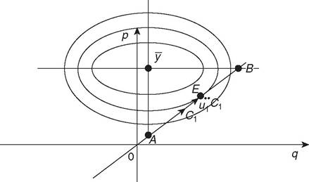
Figure 1.2 Flexible-target approach.
(Source: Acocella, Di Bartolomeo and Hughes Hallett 2013)
We can still represent the targets in the same space. Figure 1.2 shows concentric ellipses around the first best point and indicates a sequence of loss levels which diminish as we go towards the centre of the ellipses. If Q = I, these ellipses will become concentric circles.
Of course, to reach the centre of the ellipses or circles would represent the solution in the case where the system is actually Tinbergen controllable.
In contrast, we need to consider the case where only one instrument is available, as described in Figure 1.2.If only one instrument is available, the policymaker cannot achieve his or her first best target value y. But this instrument can still be set to achieve either the desired value for the quantity (point A), or prices (point B), or for a range of points in between. Clearly both A and B are suboptimal since they fail to find the lowest possible loss, given the constraint. The optimal policy, marked as u1** here, corresponds to the point of tangency between the innermost reachable ellipse and the line defined by slope C1. At point E, the marginal rate of substitution is equal to the policy multiplier (in substance, the marginal rate of transformation of q into p), and thus the policymaker’s marginal benefit equals his or her marginal cost.
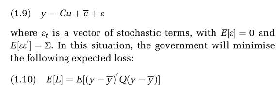
1.6.3 Uncertainty and Certainty Equivalence
In examining the impact of uncertainty on policy choice, consider first the case of a source of uncertainty that can be expressed as the additive error vector (‘additive uncertainty') only and then the more difficult one where it leads to ‘multiplicative uncertainty'. The first case takes place when the government is not sure about the transmission of the effect of its instruments (u) on its targets (y) as uncertainty about the non-controllable variables is present. Formally,
In terms of expectations, the condition that solves the government's problem does not differ from the optimal policy under certainty. Thus, we can state that if the only source of uncertainty is additive, then the optimal policy of the government is to behave ‘as if' everything was known with certainty given the expectation (‘certainty-equivalence principle').18
Certainty-equivalent decisions require no knowledge of the distribution functions of the random variables beyond their conditional means.
However, the larger the dispersion of stochastic terms for a given mean, the greater are the risks about the realised target values. Hence, certainty-equivalent decisions reflect a risk-neutral attitude; they are unaffected by risk aversion or indeed by any term reflecting the degree of uncertainty. This is their chief disadvantage: they do not react to risk or the degree, skew or possibility of catastrophic outcomes (fat tails) in the random variables. However,18
The resultwas first proposed by Tinbergen (1952) and then Theil (1958).
different ‘risk-sensitive’ or robust decision rules have been suggested (see Holly and Hughes Hallett 1989 and references therein).
‘Multiplicative uncertainty’ takes place when there is uncertainty about the parameters of the model. In this case. the policymaker cannot behave as if uncertainty does not exist. As a result, under multiplicative uncertainty, policymakers will usually tend to be more cautious in the exercise of policy and express a less vigorous response to disturbances. The decisions that minimise E∣L∣ would actually be
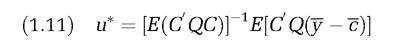
which in general gives values for the instruments that are very different from those offered by the ‘first-order certaintyequivalence solution’ unless variances and co-variances of the uncertain parameters (and the co-variances of those parameters with exogenous shocks) are small (for indications on how to deal with multiplicative uncertainty, see Acocella, Di Bartolomeo and Hughes Hallett 2013).
For brevity, we omit consideration of controllability in a dynamic setting, possibly in situations of uncertainty, instrument costs and linear quadratic preferences, referring the reader to Acocella, Di Bartolomeo and Hughes Hallett (2013: chap. 3).