The Neoclassical Synthesis

9.2.1. Generalizations: the IS-LM model again

In Chapter 8 we showed how attempts to normalize the Keynesian heresy began immediately after the publication of the General Theory.

Modigliani, in his article, developed Hicks’s IS-LM model with the aim of formulating a more general theory than that of Keynes.

The former differs from the ‘generalized’ model as it adopts the Cambridge quantity equation instead of the liquidity preference equation. The latter differs from it because of its hypothesis of rigid money wages. Modigliani proved that the (neo)classical model shows the usual dichotomy between the real and the monetary sectors of the economy. Flexible wages ensure that a full employment equilibrium is reached in which all the real variables depend on real factors. The neutrality of money ensures that variations in the quantity in circulation only influence the level of prices and other monetary variables. With the liquidity trap set aside as a very special case, Modigliani then showed how, given the money supply, macroeconomic equilibrium could be reached in the Keynesian model at any level of employment, so that there is no guarantee of full employment. He also showed that the hypothesis of rigid money wages caused this result. The reason is very simple: with a given money supply, the constraint on money wages becomes, in fact, a constraint on real wages. Monetary conditions determine the monetary income. Real income will vary in order to equate the marginal productivity of labour to the real wage; and there will be a different level of employment for each different wage level.

In the years after the publication of Modigliani’s article, attention was focused on the way in which wage and price flexibility manage to neutralize Keynes’s theory. It had seemed to some students that there were at least two very special cases in which not even the flexibility of wages could defeat Keynes’s arguments. One is the liquidity trap, already mentioned in Chapter 7. The other is that of the interest inelasticity of investments.

A key role in this demonstration was played by the so-called ‘wealth effect’, of which two types can be distinguished: the ‘Pigou effect’ or ‘real-balance effect’ and the ‘Keynes effect’ or ‘windfall effect’. Let us assume that unemployment exists. If money wages are flexible, they will fall, and this fall will be followed by a decrease in prices. Taking the money supply as given, the liquid balances of economic agents will increase in real terms. Then the agents will reduce their demand for money in an attempt to regain their desired liquid balances. This will cause the LM curve to shift to the right. A price fall corresponds to an increase in the money supply in real terms, and this occurs automatically with unemployment. Second, an increase in the real cash balances makes the economic agents feel richer and, as a consequence, induces them to raise their demand for consumer goods. This will cause the IS curve to move to the right, pushing the economy towards full employ­ment. Furthermore, the increase in the money supply in real terms will cause the rate of interest to fall, and this will raise the value of financial assets. The consumers, feeling richer, are able to reduce their propensity to save and this, while pushing the IS curve further to the right by increasing the multiplier, will also modify the slope of the curve. Savings become sensitive to variations in the interest rate, and the IS curve, if it was vertical, now becomes nega­tively sloped.

Finally, the addition in entrepreneurs’ financial wealth caused by interest rate reduction will induce them to spend more, even in investment activity. This is the Keynes effect, which implies an increase in the interest­sensitiveness of investments and therefore a further change in the slope of the IS curve.

It was Patinkin who settled these results within a general-equilibrium model, and who, in the abovementioned book, managed to generalize the generalized neoclassical model of Hicks and Modigliani. The new general­ization consisted, on the one hand, of the introduction of a fourth market, that of financial assets, besides those of ‘national product’, money, and labour, and, on the other of the introduction of a new variable in the supply and demand functions of all four goods, i.e. the price level. This variable enters into the supply and demand functions of labour together with money wages, in such a way that only real wages count, thus eliminating any pos­sible ‘monetary illusion’. It enters the demand functions for goods, money, and bonds as well as that of the supply function of bonds, as a deflator of liquid balances, so that only their real value counts. It is not surprising that in this model the neutrality of money and the usual neoclassical dichotomy are confirmed. The beauty of Patinkin’s theory is in its clear elucidation of the hypotheses on which his conclusions depend. The two principal hypotheses concern the absence of monetary illusion and the perfect flexibility of prices on all markets. There seems to be no hope for Keynes: if interpreted within a general-equilibrium model, his general theory dissolves into nothing.

Together with this kind of generalization work, the economists of the neoclassical synthesis carried out a series of investigations on specific aspects of Keynesian theory with the aim of correcting some of its particular flaws, refining some of its peculiar theses, and adjusting the latter to the results of empirical research.

9.2.2. Refinements: the consumption function

The consumption function played a fundamental role in Keynes’s theory, as it allowed the identification of a simple relationship between consumption and income from which a measure of the marginal propensity to consume and the multiplier could be obtained. It is important that such a function is stable, in the sense that its parameters do not vary significantly when the magnitudes of the variables change. Only if the multiplier is stable can the Keynesian procedure for explaining the variations in income and employ­ment by autonomous expenditure be considered legitimate. The Keynesian consumption function in its simplest form is:

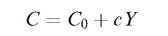
where C₀ is a constant, C represents consumption, and Y the disposable income (i.e. the income earned net of taxes). In this function, the average propensity to consume, C/Y, is higher than the marginal propensity, c. It is obvious that such a function cannot hold true in the long run, nor can it be applied to a long period; otherwise, it would lead to negative aggregate savings corresponding to low income levels.

Another function which holds true in the long run, as Simon Kuznets (1901-85) showed in Uses of National Income in Peace and War (1942), is a function of the following type:

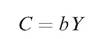
in which the marginal propensity to consume, b, coincides with the average one and is higher than that measured by c.

A simple and reasonable explanation of the differences between short-run and long-run functions was offered by the ‘relative income’ hypothesis, which was proposed by Dorothy Brady and Rose Friedman and then developed by Duesenberry. According to this hypothesis, family consump­tion is a function of ‘relative’, besides absolute, incomes. Poor families have an average propensity to consume which is higher than rich families, so that cross-section data show a decreasing average propensity to consume. When the national income increases, without any change in its distribution, the consumption of all families will increase in the same proportion, in such a way that the distribution of consumption will also remain broadly constant. In this way, the national average of the average (family) propensities to consume can remain constant through time. In other words, with a variation in the national income the short-run consumption function would shift upwards along a long-run function. This explanation, despite its reason­ableness, did not have a great deal of success, perhaps because, being too faithful to the Keynesian spirit, it did not attribute great weight to the need to find a microeconomic foundation based on the assumption of maximizing behaviour of the consumers, or perhaps because neoclassical economists love sociological reductions less than psychological ones, or perhaps for both reasons.

A suggestion which achieved more success was that advanced by Tobin in 1951, when he included wealth among the arguments of the short-run consumption function. His suggestion was taken up by Modigliani and Brumberg, who, in ‘Utility Analysis and the Consumption Function: An Interpretation of Cross-Section Data’ (1954), put forward the so-called ‘life-cycle’ hypothesis. The new theory underwent various modifications and refinements in the debates that followed, but few substantial changes. It can be presented succinctly in the following way. In the presence of an additive utility function, and with decreasing marginal utility, consumers try to dis­tribute their consumption in a uniform way over their life span, so as not consume too much when they earn a lot and too little when they earn little. Thus, during their working years they save so as to accumulate wealth to use when they are old and when they have stopped producing income. The consumption function has two arguments: wealth, W, and the life-long expected income, Y_e, which is what the individual expects to earn on average, annually, over his life. The function will be:

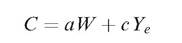
Kuznets’s problem is easily solved if the ratio between wealth and disposable income and between life income and disposable income are assumed con­stant. Then the average propensity to consume, C/Y = aW/Y + cY_e∕Y, will be constant. However, this will only happen in the long run, when it is legit­imate to assume that the wealth-income ratio is constant. In the short run, on the other hand, such a relationship will oscillate considerably, and with it the average propensity to consume.

Not too dissimilar to this is Milton Friedman’s theory of ‘permanent income’, formulated in A Theory of Consumption Function (1957). Permanent income is defined as the present value of future wealth. As this is unknown, the evaluation of permanent income depends on the expectations of the consumers. Assuming adaptive expectations, permanent income, Y_p, can be calculated as a weighted average of the incomes earned in past years—in practice, as an average of current incomes earned in the two years of the most recent past, Y and Y~₁:

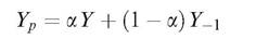
with 0 < a < 1. The long-run consumption function will depend on per­manent income, and will be: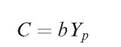

However, in the short run the current income will differ from the permanent one because of a random transitory component. If it is lower, the short-run average propensity to consume will be greater than the long-run one, and vice versa. Thus, the marginal propensity will be lower than the average propensity, and this can be explained by the fact that individuals do not know whether the variations observed in their current incomes will be maintained through time or are only transitory. Therefore, by regressing consumptions on current incomes the following function should be obtained: 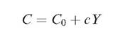which is the same as the simple Keynesian consumption function. But Friedman has derived it from a theory which explains it as a highly unstable function. The parameters can vary substantially with changes in current income, as this includes a strong random and transitory component. We will see later which important role was to be assigned by Friedman, in the attack on Keynesian theory, to the instability of the consumption function.

9.2.3. Corrections: money and inflation

Another field in which the theorists of the neoclassical synthesis went beyond Keynes was that of the theory of the demand for money. In Keynes’s model, speculators carry out a key role. They speculate on the changes in the value of financial assets, forming expectations based over an extremely brief period and paying no attention to the fundamentals which should govern share prices. Such expectations assume the form of forecasts with regard to the expectations of others and, on certain occasions, when the markets are dominated by phenomena of mass psychology, they become self-fulfilling,

producing instability and abrupt crashes. If the demand for money is dominated, or is influenced to a substantial degree, by speculation of this type, it will be affected by drastic changes or unexpected jumps following variations in the opinions of the speculators. As these opinions can also vary unpredictably in relation to interest rate changes, the demand function for money is extremely unstable, and is unable to provide reliable support to monetary policy. In fact, Keynes was rather sceptical, not only about the efficacy, but also about the implementation of discretionary monetary policies.

The neoclassical revision of Keynes’s theory of the demand for money had three main aims:

(1) to expel destabilizing speculation from the theory;

(2) to find microeconomic foundations capable of linking the aggregate demand for money to some form of individual maximization behaviour;

(3) to construct a stable function of the demand for money.

An attempt to account for the existence of a stable relationship between the transaction demand for money and the rate of interest was made by Baumol in 1952. By applying the theory of inventory decisions to the demand for money, Baumol demonstrated that the transaction demand depends on the volume of transactions, on the costs that must be sustained to convert short­term assets into money, and, above all, on the rate of interest. This occurs because the cash balances held by firms for the normal running of business represent a cost in terms of the yields forsaken for not having invested the wealth in less liquid assets. When the rate of interest increases, this oppor­tunity cost also increases and, all other conditions being equal, the companies are induced to reduce their cash balances. The transaction demand for money is therefore a decreasing function of the rate of interest.

More ambitious attempts to find a microeconomic foundation for mon­etary theory were made by Hicks and Tobin. In the 1950s a theory of portfolio selection was developed, about which we should mention at least two works by Harry Markowitz, the article ‘Portfolio Selection’ (Journal of Finance, 1952) and the book Portfolio Selection (1959), and one by Tobin, ‘Liquidity Preference as Behaviour toward Risk’ (Review of Economic Studies, 1958). Tobin directly tackled the problem of the speculative demand for money, and solved it by reducing it to a problem of choice in respect to risk. The holding of non-liquid assets gives a return, which is the sum of the interest and the capital gains, that cash cannot give. Economic agents formulate expectations in regard to possible capital gains, and specify these in the form of a frequency distribution. They admit the possibility that actual values might differ from expected ones, and attribute to each of these pos­sibilities a subjective probability. Tobin assumed, for the sake of simplicity, a normal distribution, and took its mean as a measure of the expected value and its standard deviation as a measure of risk. Given the current rate of interest and the expected capital gain, the expected returns from the investment will be an increasing function of risk. As the percentage of wealth invested in non-liquid assets increases, so do the returns, but also the riski­ness of the investment. The investor will have preferences concerning the way to combine returns and risk. His problem is therefore reduced to one of maximizing satisfaction, and the way in which he divides his wealth between money and non-liquid assets will depend on his risk aversion. In order to induce a typical investor, who is assumed to be averse to risk, to increase the demand for non-liquid assets and therefore to decrease the demand for money, it is necessary to increase the interest rate. Thus, the speculative demand for money is a stable decreasing function of the interest rate.

In ‘A General Equilibrium Approach to Monetary Theory’ (1969) Tobin extended the theory of portfolio choice to the general case in which agents must choose among a vast range of financial assets. Among these he included real capital stock. Furthermore, he introduced a new variable, q, which he defined as the ratio between the market valuation of a firm and the replacement cost of its capital. This is the origin of the famous ‘q-theory’ of accumulation. When q increases, firms have no difficulty in finding external finance, which is abundant and cheap; therefore, real investments will increase. When q decreases and the stock market valuation becomes lower than the replacement cost of capital, firms which wish to invest will find it more advantageous to buy other firms or shares in other firms on the stock exchange, rather than increase their real investments. Thus, investments are an increasing function of q. It is this q that should appear in the IS-LM model, rather than a generic ‘rate of interest’. It remains true, however, that q depends, in any case, on the decisions of the monetary authorities about interest rate levels and structure. Therefore, the possibility that investments are insensitive to discretionary monetary policies must be excluded.

Another field of investigation in which the neoclassical synthesis tried to improve upon Keynes was the theory of inflation. On this subject Keynes had formulated a precise theory as early as the Treatise. And he remained basically faithful to that theory even after the publication of the General Theory; so much so that he reproposed it almost unchanged in How to Pay for the War (1940). He believed that inflation depends on the excess of aggregate expenditure over real output, and therefore that it becomes a relevant problem only in the presence of full employment. In such a situ­ation, an excess of aggregate demand increases profits and initiates a cumulative inflationary process which, by modifying the distribution of income in favour of the capitalists, will continue until savings have increased to the level necessary to finance investments. A corollary of this theory (which, however, was developed by post-Keynesians rather than by Keynes himself) is that, in an unemployment situation, inflation cannot be explained by the forces of demand, but only by the impulses coming from costs.

This dualistic theoretical stance, with pure demand-pull inflation in periods of full employment and pure cost-push inflation in the presence of unem­ployment, did not seem very elegant, and was disliked by many economists; and as soon as a pretext appeared on which to reject it, all the neoclassical Keynesian economists seized the opportunity. The pretext was offered by Alban William H. Phillips, who, in ‘The Relationship between Unemploy­ment and the Rate of Change of Money Wage Rates in the United Kingdom, 1861-1957’ (1958), set out the results of an empirical investigation from which emerged the existence of a decreasing function between the growth rate of money wages and the rate of unemployment. The orthodox theoretical explanation of the ‘Phillips curve’ was given by Richard George Lipsey. Wages change as an increasing function of the excess demand for labour. The rate of unemployment reflects this excess demand. In this way, the Phillips curve is reconciled with the orthodox theory of wages, except for the fact, which was later to turn out to be crucial, that it is not the variations in real wages but those in money wages that it makes depend on the excess demand.

9.2.2. Simplifications: growth and distribution

The final step that still had to be taken to complete the reabsorption of Keynes into the neoclassical theoretical system was to show that the interest rate, while being influenced by monetary forces, remained regulated by real forces; and that, in the end, it was possible to reduce it to be precisely what Keynes had denied it was, i.e. the price of the services of real capital, or the equilibrium price of savings and investments. Hicks and Modigliani, in the two abovementioned articles on the IS-LM model, had already tried to reach this result. But that model, based as it was on the hypothesis of temporary equilibrium (with a given capital stock) did not lend itself to this purpose. To make interest the equilibrium price of the services of capital, it is necessary to be able to link it to the productivity of capital and make it depend on the proportions in which capital is utilized in relation to other factors. Besides this, it is essential that these proportions can be linked to the decisions of optimizing economic agents, as the equilibrium is a situation in which the individuals have maximized their own objectives. Finally, the capital stock cannot be taken as given; and it is concept of long-run equi­librium that must be referred to. These objectives were reached (at least it seemed so at that time) by the neoclassical growth models.

We will ignore the vast amount of literature which appeared on the subject in the 1960s, and limit ourselves to mentioning the first and simplest of these models, that formulated by Solow in ‘A Contribution to the Theory of Economic Growth’ and by T. W. Swan in ‘Economic Growth and Capital Accumulation’, both published in 1956. However, it is important to point out that, a year before, Tobin had already drawn the essential lines of this model in ‘A Dynamic Aggregative Model’.

The explanation of the interest rate by the marginal productivity of capital was only one of the birds to be killed with Solow’s stone. Another was the solution of a basic problem concerned with growth which had emerged from the Harrod-Domar model: that of the possibility for a capitalist economy to grow at the ‘natural’ rate, ensuring the maintenance of full employment. The neoclassical economists set aside the problem of stability from the very beginning by assuming that the economy always grows at the warranted rate. Then the problem of natural growth was solved by adding to the three basic equations of the Harrod-Domar model (see section 7.1.6) an aggregate production function of the type Y = F(K, L), in which Y represents the national income, K capital, and L labour. In Chapter 11, when we consider the debate on the theory of capital, we will discuss the analytical and theoretical difficulties inherent in the concepts themselves of an aggregate production function and aggregate capital. Here we will ignore them by treating capital as if it were jelly.

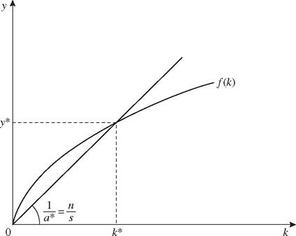
If constant returns to scale are assumed, the production function can be rewritten as y = f (k), with y = Y/L and k = K/L, as shown in Fig. 11. Now, it can be proved by making adequate hypotheses on the form of the production function that, given the propensity to save, there is a unique capital—output ratio which ensures equality between the warranted rate of growth and the natural rate, n. In other words, α*, the full-employment capital—output ratio, is determined endogenously in such a way as to guarantee the equality s/a* = n, or 1/a* = n/s.

The solution of the Harrod-Domar problem was achieved by treating the capital-output ratio as a variable, instead of as a datum. The economic meaning of this solution must be found in the fact that, as the capital-output

ratio is variable, entrepreneurs will choose it with the aim of maximizing their profits. The techniques will change in response to variations in factor prices. At any moment, if an unemployment situation occurs, the flexibility of real wages guarantees a reduction in the cost of labour necessary to induce the entrepreneurs to modify the techniques in such a way as to increase the demand for labour. Unemployment can only be temporary and frictional. In equilibrium, the wage rate will be equal to the marginal productivity of labour, and the economy will grow with full employment.

In the same way, any monetary disturbance which alters the rate of interest will induce entrepreneurs to modify their demand for capital in such a way as to equate its marginal productivity to the cost of finance. Thus equilibrium on the capital market will be ensured by an interest rate which rewards the productive services of capital, being equal to its marginal productivity.

The persuasiveness of this model was also linked to the fact that it seemed to account in the simplest way for a historical phenomenon which Keynes would have had difficulty in believing in and which the Harrod-Domar model was incapable of explaining: the ability of the most advanced capit­alist economies to grow by maintaining full employment, as had occurred in the 1950s and 1960s. This phenomenon did not lead the neoclassical economists explicitly to reject Keynes, but it did seem to justify their rejec­tion of his pessimism. After all was said and done, the capitalist economy seemed able to look after itself, so that Keynesian economic policies were not needed to cure any incurable illness. At most they could be called up to correct some imperfections, for example when trade unions insisted in raising wages. In general, however, they were only needed to ‘fine-tune’ economic growth, and to minimize oscillations, so as to allow the ‘invisible hand’ to work with ease. On the other hand, as they were short-run policies, nothing more could be expected of them. In the same way in which Keynesian theory did not damage the neoclassical theoretical framework in any essential way, Keynesian policies would not impinge upon the operation of the market.

9.3.