Alternative Interpretation: Trader Dynamics to Generate Financial Complexity

This section is inspired by Philip Maymin’s ingenious demonstrations in the Wolfram Demonstration Project. He attempted to formulate a single autonomous engine, based on the application of automata, to recreate complex stock price fluctuations.

Maymin has focused on the actual aspect of traders’ decisions in terms of the combining of multiple layers: actions, mind states, and memories of traders and the market. The environment, here the market, is generated by a rule, but not by factors such as drift and other random factors that often appear in statistical time series analysis. If the market is rising, there are two possible kinds of action. One is a trend-follower action: to buy rising stocks. This may reflect a bearish or pessimistic mind. The other is the contrarian action to sell on the way up, or to buy on the way down. This may reflect a bullish or optimistic mind.

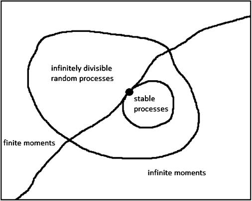
Fig. 6.11 Illustration scheme of classes of random processes. Note: The solid circle denotes the stable Gaussian process. Cited from Swell (2011, Fig. 3) (Swell 2011, p. 4, said: “Price-influencing events may be normally distributed, but the likelihood of said events being reported in the news increases with the magnitude of the impact of the event. For the latter distribution, one can factor in the tendency for the media to simplify and exaggerate. Multiply the normal distribution by the distribution according to the likelihood/duration/impact of news reports and one has a much fatter- tailed distribution than a Gaussian.”)

The resulting behavior of the trader depends on the mind state, whether bearish or bullish.

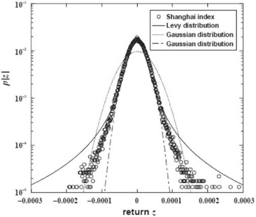
Fig. 6.12 Shanghai index. Cited from Fig. 4 of Swell (2011)

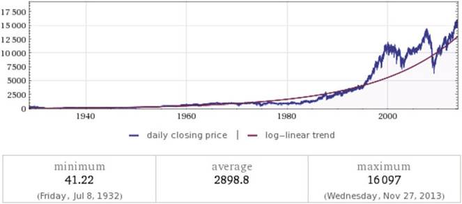
Fig. 6.13 All data from the Dow Jones Index. Source: Wolfram Alpha. http://www. wolframalpha. com/input/?i=dow+jones

Figure 6.16 shows this idea in more detail.

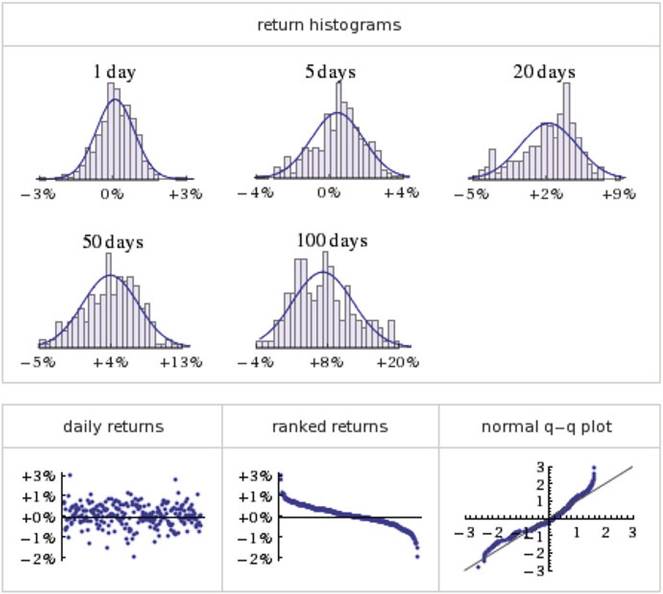
Fig. 6.14 Last year’s distributions of the Dow Jones Index on Dec 14, 2013. Source: Wolfram Alpha http://www.wolframalpha.com/input/?i=dow+jones

6.4.1 Rules to Be Specified

Even if we assume the simplest dealing, we would require several behavioral rules to achieve buy, sell and hold, taking into account the market state as well as a trader’s memory.

1. Action rules depending on the mind state:

a. Internal rule

b. Shift rule (transducer)

2. Look-back rule: the trader’s memory of action associated with the hysteresis of the market

In the case of two actions {buy, sell}, two states {bearish, bullish}, and {three- period memory}, there are 256 possible rules, including overlapping ones. Some

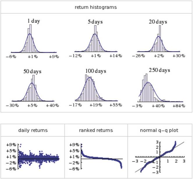
Fig. 6.15 The last 5 years’ distributions of the Dow Jones Index on Dec 14, 2013. Source:

Wolfram Alpha http://www.wolframalpha.com/input/?i=dow+jones

rules may be more important than others. We usually have two rules for state of mind: one that gives the internal rule, and one the shift rule between the different states of mind. In reality, however, there are many combinations of mind state and market state, as well as actions of buy and sell.

The investor is modeled using an iterated finite automaton with only two states: an optimistic contrarian state and a pessimistic trend-following state. The trader starts each day in the optimistic contrarian state, which sells on upturns and buys on downturns, and remains in this state as long as the market keeps going up.

We take first a simple example. Maymin (2007d: Caption comment) described this model as:

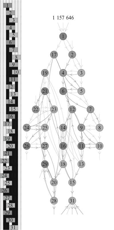
Pick the rule he follows and the initial conditions for the first three days of the week. The trader looks back over the past three days in considering what to do. The big circles are states, like the emotions of the trader. He always starts in state 1 and then follows the arrows that correspond to the market movement (UP or DOWN) of the day under consideration. The yellow state is the one he was in when he started thinking about the day in question,

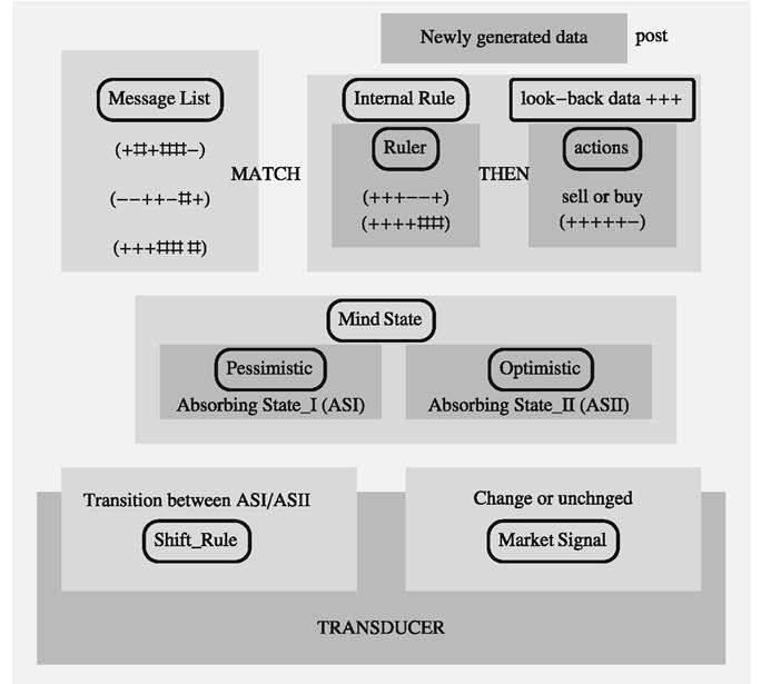
Fig.

and the one with the square in it is the one he will move to, based on the yellow arrow that he follows. His “current thinking” is shown on the yellow arrow, too (BUY or SELL), but he only makes his final decision when he has reached the last day that he considers.

• Action rule

Internal rule of the trader mind: In the bearish state, the trader sells when the market is UP. In the bullish state, the trader sells when the market is DOWN.

Shift rule of the trader mind: Shift to the bearish state so that the trader buys when the market is UP. Shift to the bullish state so that the trader buys when the market is DOWN.

Look-back rule

The last three units of time are used for the look-back.

According to Maymin, we can imagine the initial conditions shown in Fig. 6.17.

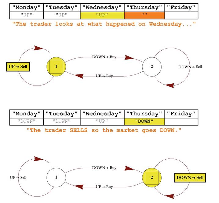
Fig. 6.17 Internal rules in different initial conditions

The investor follows these transitions by looking at the past few days of price changes, starting with the most recent day. The decision to buy or sell is modeled as his current thinking as he goes through the past few days, and once he reaches the last day of his look­back window, he makes his final decision to buy or sell. The next day, he starts all over.^[73] (Maymin 2007a: Details)

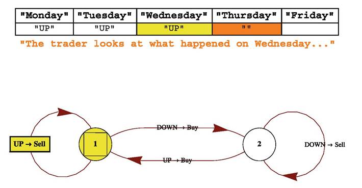
Fig. 6.18 A shift rule sensitive to the market change

In this instance of, the transition of the market will be shown in terms of the transducer finite automata:

{state1, input} → {state2, output} (6.41)

Here, the trader is pessimistic and remains in this state as long as the market keeps going down.

In the left-hand side of Fig. 6.17, “[o]n the first downtick, it transitions to the other state, the pessimistic trend-following state. This state is trend-following because it buys on upticks and sells on downticks”.

In this rule:

state 1 is characterized as an up-absorbing state. state 2 is characterized as a down-absorbing state.

Consequently, the rule could give the following reduced rule:

1. If the preceding two events are the same, i.e., both up or both down, the trader will sell.

2. If the preceding two events are different, i.e., one up and one down, the trader will buy.

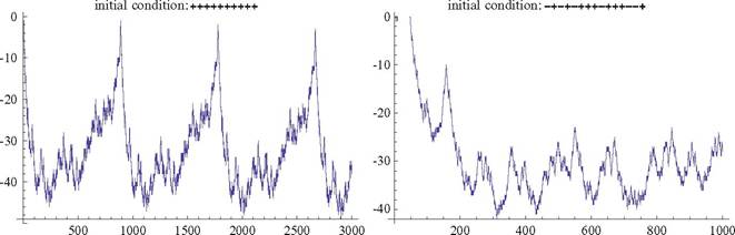
Fig. 6.19 The same trader with ten look-back windows and price motions under different initial conditions

6.4.1.1 An Alternative Interpretation Based on Tick Data

If each event is replaced by a tick,^[74] Maymin suggests:

An investor observes two consecutive ticks. If they are the same sign, i.e., either both up or both down, then he sells. Otherwise he buys. However, his order does not take effect for w — 1 ticks. Put another way, his orders face a delay of w — 1 ticks, so the minimal model formalizes an investor who looks at consecutive ticks to decide his position and faces a short delay either in mental processing or order execution (Maymin 2011a, p. 10).

Here the first component is the state, 1 (bearish) or 2 (bullish). The second is the trader’s action keeping up with the market state:

1: buy at up

0: sell at down

The trader will follow the shift rule as shown by ) (see Fig. 6.18).

We now extend the look-back windows to 10 days or ticks, obtaining a new time series (see Fig. 6.19).

6.4.1.2 A Generalization of the Simplest Trader Dynamics

Maymin proposed to define the domain of his speculative financial market as:

An investor with s internal states and k possible “actions” with base b and having a look­back window of w days is modeled as an iterated finite automaton (IFA).

Employing the Wolfram IFA numbering scheme, the IFA is run as:

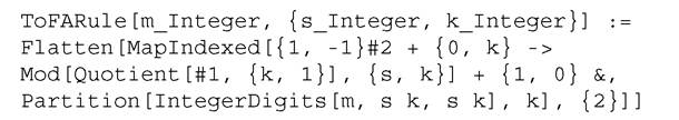
s represents the state of mind of the trader, which is sometimes bearish, sometimes bullish. k represents the action of dealing, usually “buy”, “sell”, or “hold”, although it may be accompanied by the “limit order” or the “market order”. For simplicity, we assume dealing is to the market order only, because this is often genuinely possible. When k = 2 (Maymin 2011a), the possible actions are buy and sell. Maymin also proved that the possible actions are buy, sell, and hold if k = 3. He introduced a scale of strength of buy or sell, where the possible actions are buy, buy more, sell, and sell more, if k = 4.^[75]

In general, if k is even, the possible actions are k/2 types of buys and k/2 types of sells, with differing strengths. If k is odd, the possible actions are the same as for k — 1 with the additional possibility of doing nothing, i.e., hold.

There is a basic property of these new trader dynamics, that “[the trader] never learns his own rule”. In this modeling, however, the trader is based on “technical analysis”, and will trade in reference to a self-chosen technical indicator (Maymin 2011a, p. 4). In Maymin’s simple model, the trader will not change rule until there is a big loss. It follows that:

From his point of view, he put in an order to buy and was simply unlucky enough not to have been filled before the market moved away. This happens to him every day, whether he wants to buy or sell (Maymin 2011a, p. 4).

6.4.1.3 How Do the New Traders’ Dynamics Differ from Previous Models?

The new dynamics proposed by Maymin decisively differ from previous ideas as they contain rules. In many game theoretic formulations, the players are allowed to change moves by checking the ongoing development of the price. In this case, we specify that the trader can decide his market order, i.e., whether he can buy or sell, by looking back at the preceding price series. In other words, his decision depends on his previous memory. Given the preceding time series DOWN, UP, UP, the trader

Table 6.1 Transitory evolution of memory in traditional trader dynamics

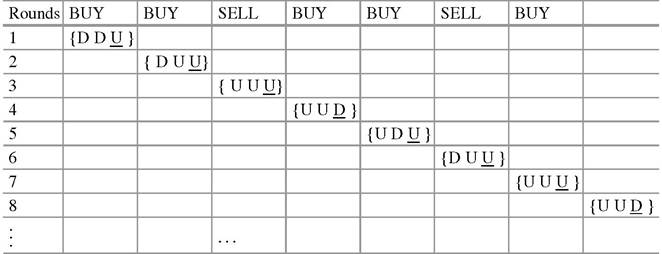
Note: Underlined letters indicate the current event on Up or Down.

Fig. 6.20 A time series generated

will buy because of an expectation that the price will go up further. However, his memory is limited to three elements of the last price movement (Table 6.1).

The consequence may not differ from the new results, but the choice of the shift rules for mind transition could give rise to a big change in the price series (Fig. 6.20).

6.4.1.4 Maymin’s Justification for the Simplest Trader Dynamics

In the financial market, as described by Maymin, there is no need for multiple traders to create complex price fluctuations. We assume only the initial price ahead of the opening price quotation, on which the trader can act. The preceding price series motivates the trader to make further orders. Maymin (2007a,b,c,d; 2011a,b) gave this price information in the up and down form: {up, down}. Even this price series is created by the trader himself. The simplest model uses only a single trader, but this may be replaced with the point that in the preceding session, some trades were made, whether our particular trader was involved or not. After moving to the opening price,^[76] only one trader will continue to give further orders. In the futures market, self-dealing is acceptable, and in a double auction, it is possible to have simultaneous moves of buy and sell, usually called the day trader method. It is therefore possible to assume a sole agent in the market. Here the interactive effects caused by different agents may not be explicit but the interaction between buy and sell definitely emerges. We can therefore employ the single market simulation to investigate how and why a complex price fluctuation can be created. The market dealings allow moves of only sell, buy or hold, although there are also two kinds of limit order and the market order, as shown in Chap. 4. A trader may sometimes secure his profit by executing market orders. We therefore take an example of a single trader with market orders. This setting may be reasonable if we comply faithfully with the basic properties of the financial market.

This market will be reflected by the emotions of the trader, which essentially coincides with Lux (2009) and Hawkins (2011), where the market could be characterized by the simulation method of emotional interaction irrelevant to the real economy. This is an essential property of the financial market. In the event, through this kind of experiment, we can recognize the new proposition:

Proposition 6.1. The market is not capable of creating price fluctuations. Instead, the situation is the other way round. A trader, even if there is only one, can create the market, which is simply an institutional arrangement.

It is important to understand that the market in itself is not capable of creating anything. The agent does not have to be human. In high-frequency trading (HFT), the main agents are algorithmic ones. This proposition does not imply that human behavior can create a market fluctuation.

Another important feature of the financial market could be compatible with the sock puppet idea.

Proposition 6.2. A monologue, i.e., a single trader dynamic, can move the market, whether the action is judged illegal or not.^[77]

A sock puppet means “an online identity used for purposes of deception”.^[78] We assume that a sock puppet is the single trader in our market, and call the single trade dynamics required to generate a complex stock price fluctuation “sock puppet dynamics”.

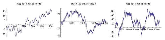
Fig. 6.21 Using 15 look-back windows

In dealings, the trader must have a strategy. The standard classical strategies are still applied in the market, although they date back to the era of the classical stock exchange. They may be used not only by human agents but also by machine or algorithm agents, and as we saw in Chap. 4, the random strategy or zero-intelligent strategy can work well.^[79]

The trader can be given alternative options from the same past history, includ- ingtowards the trend or against it, either the trend strategy or the anti-trend strategy. Either way, the decision could be canceled out before the simulation in either the classical auction or HFT. Throughout, the trader is never required to hold to the first choice of strategy, but can switch strategy either emotionally or intelligently. Needless to say, in the market, an intelligent strategy will never guarantee profits, even if the strategy is very sophisticated. Random strategies, on average, minimize the total loss because of naive risk management.

6.4.2 Complexities in a Dealing Model of an Iterated Finite Automaton

First we need to define complexity. With a look-back window of w with k possible market movements each day, there are only k^w distinct possible price histories on which the trader bases a decision. After k^w days of history, the time series of price changes must have cycled. A complex series is one that takes a long time to cycle, and a simple series cycles quickly.

For example, a rule that always buys will cycle in a single day. Even though the price continues to rise to a unique level each day, the changes are constant. Here, using Maymin’s simulator,^[80] we can verify some findings of complex price motions, a periodic motion (see Fig. 6.21).

6.4.2.1 Redundancies and the Depth of Logic Contained in a Complex System

This modeling has definitely generated complex price fluctuations. In general, however, it may be that there are actually not so many long complex price motions. Such an observation is usually true of other chaotic movements. Sequences with low complexity are more likely than those with high complexity, as we saw with DNA in a previous chapter (Mainzer 2007, p. 156).

Redundancies and the depth of logic contained in a complex system Redun­

dancy mediated by a coincidence may bring something new. A combinatorial rearrangement found among redundancies suggests the potential for a new idea. If each program to generate a given consequence is smaller, the number of steps calculated by these programs will be increased. As a generated system becomes more complicated, the procedure to reveal the desired system will have a deeper logic, so a simpler program can create a complex system. This is why an organism or a gene can construct a huge complex constitution with a considerably deeper logic in spite of its simple procedure.

Recently, complex systems have often been analyzed as complex networks, but the present form of network analysis is insufficient because of the depth of logic and information. Network analysis gives useful findings, but does not yet have a tool to represent the depth of logic and information (Figs. 6.22, 6.23, and 6.24).

These events may be easily compared with those generated by Turing Machine (Turing 1936-37,1937). A Turing machine “consists of a line of cells known as the ‘tape’ with an active element called the ‘head’ that can move back and forth and can change the colors of the tape according to a set of rules. Its evolution can be represented by causal networks that show how the events update” (Zeleny 2005). Among 4096 rule, Zeleny produced various causal networks of the next kinds: (1) repetitive behavior, (2) a binary counter, (3) a transient, (4) a stable structure from a random initial condition, and (5) arrows jumps backwards and forwards several levels. For reference, we reproduce the case (5) of three states with two colors (Fig. 6.25):

Here the change of mind state of the trader dynamics may correspond to the head change of Turing machine. Thus it evolution will be similar to the evolution of mind state in the trader dynamics. Thus we may expect that our trader dynamics can make a causal complex network. It may be also natural to argue NP (Non-deterministic Polynomial) complexity in non-deterministic Turing machine (Maymin 2011b).

6.4.2.2 Definition of Complexity in Simple Trader Dynamics

Definition 6.2 (Maymin’s Complexity). Complexity in a k-action generated price series for a look-back window w means that the periodicity of the rule is greater than kw∕2. A rule with the maximal complexity would have a periodicity equal to the maximal periodicity (cycle length) of kw, i.e., 2w. Usually, cycle length < the maximum 2w. Generation of periodicity depends on the initial condition.

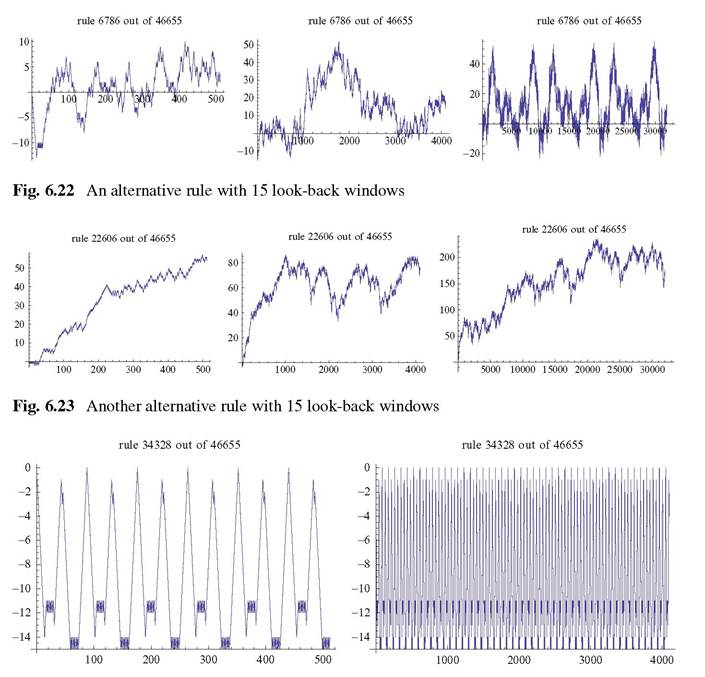
Fig. 6.24 A further rule with 15 look-back windows and periodic motion

Definition 6.3 (A Relaxed Definition). The minimal complex model must have at least two states and two actions.

Lemma 6.1 (Complexity in the Price Series).

Complexity in the price series requires s > 2 and k > 2. Cycling does not mean that the market is modeled as repeating, only that this is a characteristic of the model. We can always choose sufficiently large k and w such that the cycle length is longer than the history of the market under consideration.^[81]

Fig. 6.25 A causal network. Cited from Zeleny (2005). Note: Here the object number is set 1631

6.4.2.3 A Rapid Growth of Complexity Due to HFT in Terms of Periodicity

We found a twofold period system in HFT. Inner look-back windows accompany each time unit, with a new window denoted by w. We estimate the complexity by: kwω∕^,2 > kw/2. In our simple trader dynamics with HFT, the complexity will therefore rapidly increase.