Heavy Tail Distributions with Heavier Randomness

We have already seen a self-similarity emerging in the random walk. We now turn to heavy tail distributions.¹⁰ The term heavy tail means that there is a higher probability of getting very large values.

Many econophysicists investigated a particular subclass of heavy tail distribu­tions as power-laws, where the PDF is a power.¹¹ Such a distribution does not usually have finite variance, i.e., not all moments exist for these distributions.

^[1] 0 (1) represents a function tending to 0.

9http://mathworld.wolfram.com/ParetoDistribution.html.

^[1]See Nolan (2005, 2009).

^[1] The power law differs from the power distribution. The probability density for values in a power distribution is proportional to.v'' ¹ for 0 < x ≤ 1/k and zero otherwise.

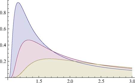
Fig. 6.7 Levy distribution: σ = 0.5, 1,2

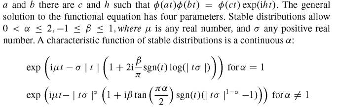
This will give rise to some technical difficulties, because of the characteristic functions for stable distributions.¹² A stable distribution is defined in terms of its characteristic function φ(t), which satisfies a functional equation where for any

This can be written in closed form in terms of the four parameters mentioned above.¹³ In general, however, the density functions for stable distributions cannot be written in closed form. There are three exceptions: normal, Cauchy, and Levy distributions (Fig. 6.7).

The probability density for value x in a Levy distribution is proportional to:

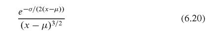
Here the Levy distribution allows μ to be any real number and σ to be any positive real number.

^[1]A linear combination of independent identically distributed stable random variables is also stable.

^[1]As already noted, the generalized CLT still holds.

6.3.1 HazardRates

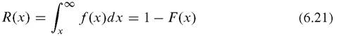
We focus on the lifetime of a person over the random variable x with probability density function f(x). The probability of surviving at least up to time x is:

dx is a small interval of time, so the probability of death in time interval dx is f(x), the probability density function. Thus the instantaneous death rate at age x, i.e., the force of mortality, is defined as:

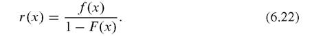
If this ratio r(x) is applied to the failure rate in manufacturing processes, it is called the hazard rate. It is clear that the distribution is possible whether the ratio rises or decreases with x ; that is, whether it has increasing failure rate (IFR) or decreasing failure rate (DFR).^[71] The lognormal distribution becomes a DFR only beyond a point, while the Pareto distribution is a DFR throughout its range.

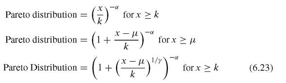
The probability density for value x in a Pareto distribution is proportional to x~^a~¹ for x > k, and zero for x < k. The survival function for value x in a Pareto distribution corresponds to:

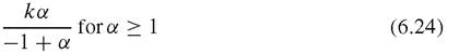
In the first form of the Pareto distribution [k, a], the mean is:

and the variance is:

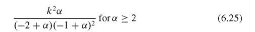
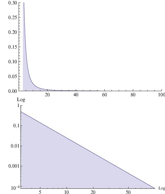
Fig.

We now derive the Pareto distribution following Singh and Maddala (2008). It is convenient to transform x into z = log x. We then find the hazard rate with respect to log x (Fig. 6.8):

Taking the negative form of the Pareto transformation, let y, z be:

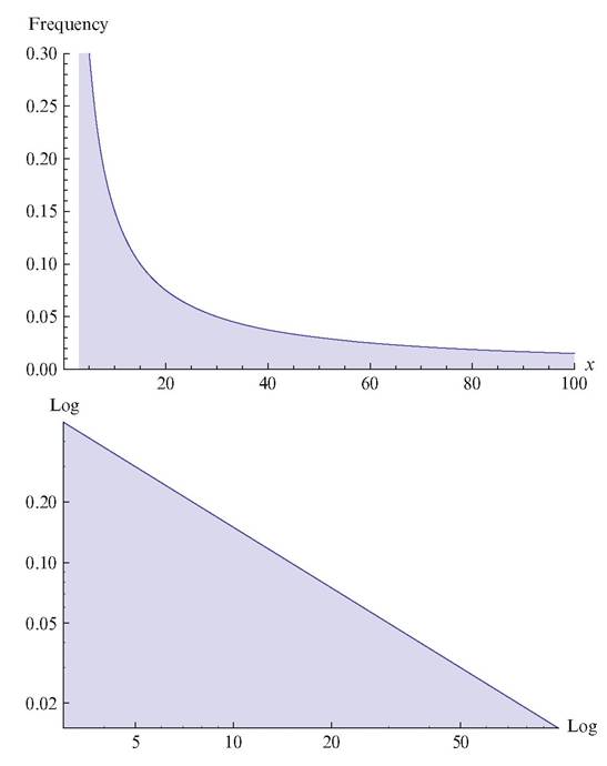
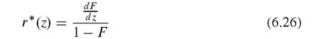
Fig. 6.9 Hazard distribution of a Pareto distribution: a = 3, k = 1.5

By the log transformation of x, y' is interpreted as the proportional failure. If we then suppose:

a is constant. The formula then implies that the rate of change of y' (the acceleration rate) depends on itself, and acceleration should move in a negative direction (Fig. 6.9).

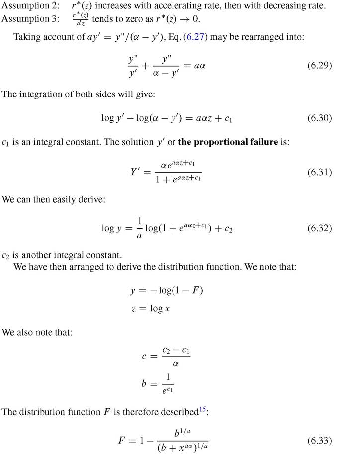
To solve this differential equation, we make three assumptions about r *(z):

Assumption 1: r *(z) approaches a constant value asymptotically.

6.3.2 An Alternative Derivation in View of Memoryless Processes

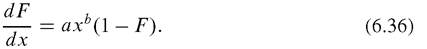
The Pareto process depends only on remaining one-sided, so dF depends on 1 — F only. Singh and Maddala (2008, p. 31) called such a process memoryless:

The most typical memoryless process may be the Poisson process:

The Weibull process is one into which memory is introduced:

The motion of x affects its behavior.

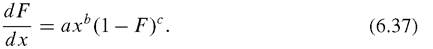
Specifically, the values of a,b,c will be verified by a concrete form of the process generating a distribution.

Now we allocate further:

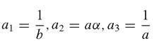
It then follows that:

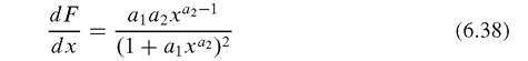
The distribution Eq. (6.38) is then rewritten into^16,17

6.3.3 Some Empirical Findings in the Market

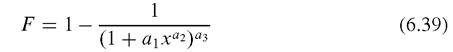
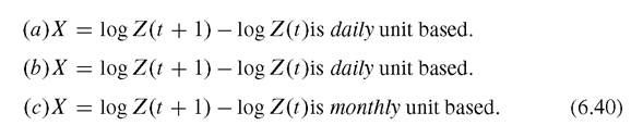
Empirical findings on the Pareto-Levy distribution were first confirmed by Man­delbrot (1963), who examined (a) the New York Cotton Exchange, 1900-1905, (b) an index of daily closing prices of cotton on various exchanges in the US, 1944­1958 (published by Hendrik S. Houthakker), and (c) the closing price on the 15th of each month at the New York Cotton Exchange, 1880-1940 (published by the US Department of Agriculture). The unit of time t in the time series is different for each. Figure 6.10 shows all three cases (a)-(c) with positive and negative axes. Notice that the variables representing the change rates in terms of logarithm are taken as differently as follows:

It may also be helpful to reproduce the scheme of random process classes given by Mantegna (2000), Swell (2011) (Fig. 6.11).

The PDF of returns for the Shanghai market data with ∆t = 1 is compared with a stable symmetric Levy distribution using the value a = 1.44 determined from the slope in a log-log plot of the central peak of the PDF as a function of the time increment. The agreement is very good over the main central portion, with deviations for large z. Two attempts to fit a Gaussian are also shown. The wider Gaussian is chosen to have the same standard deviation as the empirical data. However, the peak in the data is much narrower and higher than this Gaussian, and the tails are fatter. The narrower Gaussian is chosen to fit the central portion, but the standard deviation is now too small. It can be seen that the data have tails that are much fatter and have a non-Gaussian functional dependence (Johnson et al. 2003; Swell 2011) (Figs. 6.12, 6.13, 6.14, and 6.15).

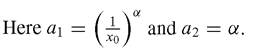
¹⁶It is clear that F → 1 as x → 1.

¹⁷See Champernowne (1953) and Fisk (1961).

Fig. 6.10 New York cotton exchange. Cited from Manderbrot (2001, Fig. 4)

6.4