Basicframework

2.1. A toy version of the Aghion-Howitt model

Asked by colleagues to show them the simplest possible version of the quality-ladder model of endogenous growth which they could teach to second year undergraduate stu­dents, we came out with the following stripped-down version of Aghion and Howitt (1992).

Time is discrete, indexed by t = 1, 2,..., and at each point in time there is a mass L of individuals, each endowed with one unit of skilled labor that she supplies inelasti- cally. Each individual lives for one period and thus seeks to maximize her consumption at the end of her period.

Each period a final good is produced according to the Cobb-Douglas technology: where x denotes the quantity of intermediate input used in final good production, and A is a productivity parameter that reflects the current quality of the intermediate good.

The intermediate good is itself produced using labor according to a simple one-for- one technology, with one unit of labor producing one unit of the current intermediate good. Thus x also denotes the amount of labor currently employed in manufacturing. But labor can also be employed in research to generate innovations.

Each innovation improves the quality of the intermediate input, from A to γA where ó > 1 measures the size of the innovation. Innovations result from research investment. More specifically, there is an innovator who, if she invests z units of labor in research, innovates with probability λz and thereby discover an improved version of the interme­diate input.

The innovator enjoy monopoly power in the production of the intermediate good, but faces a competitive fringe who can produce a unit of the same intermediate good by using χ > 1 units of labor instead of one. For χ < 1∕α, this competitive fringe is binding which means that χw_t is the maximum price the innovator can charge without being driven out of the market.

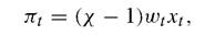
where w_tx_t is the wage bill. This monopoly rent, however, is assumed to last for one pe­riod only, after which imitation allows other individuals to produce intermediate goods of the same quality.

The model is entirely described by two equations. The first is a labor market clearing equation, which states that at each period total labor supply L is equal to manufacturing labor demand x plus total research labor n, that is: L = x_t + n_t for all t. The second is a research arbitrage equation which says that in equilibrium at any date t the amount of research undertaken by the innovator must equate the marginal cost of a unit of research labor with the expected marginal benefit. The marginal cost is just the manufacturing wage w_t. The expected benefit comes from raising the probability of success by λ ∙ 1 = λ, in which case she earns the monopoly profit π_t involved in producing the intermediate good for the final good sector. Thus the research arbitrage equation can be expressed as: 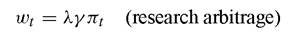where the factor γ on the right-hand side of the equation, simply stems from the fact that an innovation multiplies wages and profits by γ.

Using the fact that the allocation of labor between research and manufacturing re­mains constant in steady-state, we can drop time subscripts. Then, substituting for π_t in the research arbitrage equation, dividing through by w, and using the labor market clearing equation to substitute for x, we obtain:

which solves for the steady-state amount of research labor, namely:

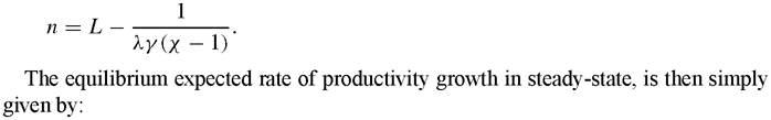
and it therefore depends upon the characteristics of the economic environment as de­scribed by the parameters λ,γ, χ, and L.

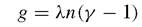
The model is extremely simple, although at the cost of making some oversimplifying assumptions. In particular, we assumed only one intermediate sector, and that labor is the only input into research. In the next sections we relax these two assumptions. We develop a slightly more elaborated version of the quality-ladder model that we then extend in several directions to capture important aspects of the growth and development process.

2.2. A generalization

There are three kinds of goods in the economy: a general-purpose good, a large number m of different specialized intermediate inputs, and labor. Time is discrete, indexed by t = 1, 2,..., and there is a mass L of individuals, each endowed with one unit of skilled labor that she supplies inelastically.¹

The general good is produced competitively using intermediate inputs and labor, ac­cording to the production function:

^[1] The model we present here is a simplified discrete-time version of the Aghion and Howitt (1992) model of creative destruction, which draws upon Acemoglu, Aghion and Zilibotti (2002). Grossman and Helpman (1991) presented a variant of the framework in which the x’s are final consumption goods and utility is log- linear. An early attempt at developing a Schumpeterian growth model with patent races in deterministic terms was presented by Segerstrom et al. (1990). Corriveau (1991) developed an elegant discrete-time model of growth through cost-reducing innovations.

where each x_it is the flow of intermediate input i used at date t, and A_it is a productivity variable that measures the quality of the input. The general good is used in turn for consumption, research, and producing the intermediate inputs.

The expected growth rate of any given productivity variable A_it is:

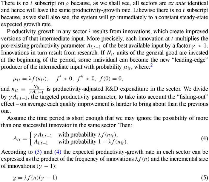
in an equilibrium where productivity-adjusted research is the same constant n in each sector. We assume moreover that the outcome of research in any one sector is statisti­cally independent of the outcome in every other sector.

The model determines research n, and therefore the expected productivity-growth rate g, using a research arbitrage equation that equates the expected cost and benefit ² More precisely, f(n) = F(n, k) where k is some specialized research factor in fixed supply and F is a constant-returns function. Since there is free entry in research, the equilibrium price of k adjusts so that the expected profit of an R&D firm is zero. Since this price plays no role in the analysis of growth we suppress the explicit representation of k and deal only with the decreasing-returns function f. (Of course the constant­returns assumption can be valid only over some limited range of inputs, since F is bounded above by unity.) of research. The payoff to research in any sector i is the prospect of a monopoly rent π_it if the research succeeds in producing an innovation. This rent lasts for one period only, as all individuals can imitate the current technology next period. Hence the ex­pected benefit from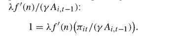spending one unit on research is π_it times the marginal probability

To solve this equation for n we need to determine the productivity-adjusted monopoly rent π_it/A_it to a successful innovator. As before, we assume that this innovator can produce the leading-edge input at a constant marginal cost of one unit of the general good.

A monopolist’s output x_it will be the amount demanded by firms in the general sector when faced with the price χ; that is, the quantity such that χ equals the marginal product of the i th intermediate good in producing the general good:

Hence:

where

Therefore we can write the research arbitrage equation, taking into account that because a monopolist is someone who has just innovated, as:

which we assume in this section has a positive solution.

³ It is easily verified that if there were no fringe then the unconstrained monopolist would charge a price equal to 1∕α, but at that price the fringe could profitably undercut her because its unit cost is χ < 1∕α.

⁴ If no innovation occurs then some firm will produce, but with no cost advantage over the fringe because everyone is able to produce last period’s intermediate input at a constant marginal cost of unity.

⁵ To see that Ó > 0 note that: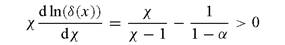

where the last inequality follows from the assumption that / < 1∕α.

The expected productivity growth rate is determined by substituting the solution of (9) into the growth equation (5). In the special case where the research-productivity function f takes the simple form:

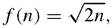
we have:

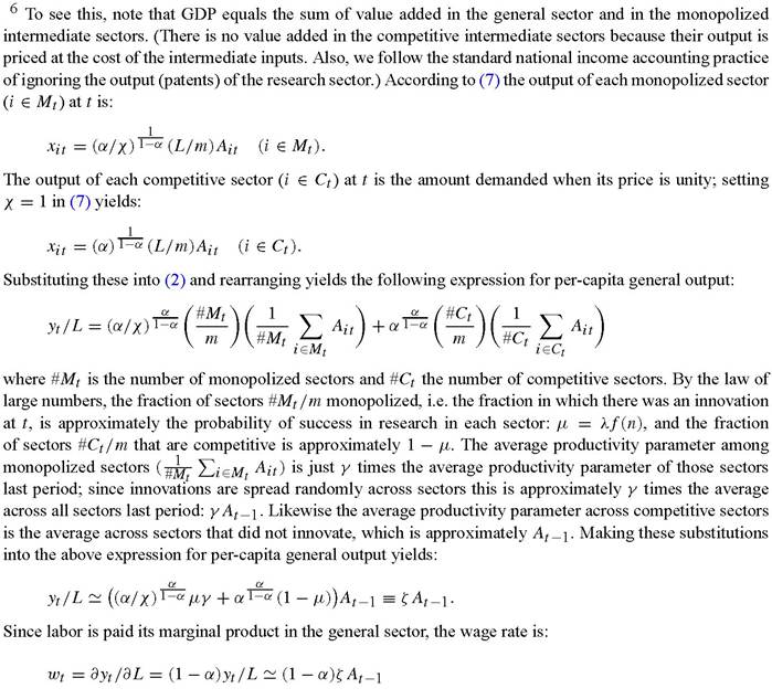
As it turns out, g is not only the expected growth rate of each sector’s productivity parameter but also the approximate growth rate of the economy’s per-capita GDP This is because per-capita GDP is approximately proportional to the unweighted average of the sector-specific productivity parameters:⁶

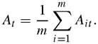
Since (a) all sectors have an expected growth rate of g, (b) the sectoral growth rates are statistically independent of each other and (c) there is a large number of them, therefore the law of large numbers implies that the average grows at approximately the same rate g as each component.

2.3. Alternative formulations

There are many other ways of formulating the basic model. We note two of them here for future reference. In the first one, as in the above toy model, the general good is used only for consumption, while skilled labor is the only factor used in producing intermediate products and research. The general good is produced by the intermediate inputs in combination with a specialized factor (for example unskilled labor) available in fixed supply. In this formulation, the growth equation is the same as (5) above, but with n being interpreted as the amount of skilled labor allocated to R&D. This version will be spelled out in somewhat more detail in Section 5.

The other popular version is one with intersectoral spillovers, in which each innova­tion produces a new intermediate product in that sector embodying the maximum A_{t -1} of all productivity parameters of the last period, across all sectors, times some factor γ that depends on the flow of innovations in the whole economy. The idea here is that if a sector has been unlucky for a long time, while the rest of the economy has progressed, the technological progress elsewhere spills over into the innovation in this sector, re­sulting in a larger innovation than if the innovation had occurred many years ago. The model in Section 3 is a variant of this version.

2.4. Comparative statics on growth

Equation (10) delivers several comparative-statics results, each with important policy implications on how to “manage” the growth process:

1. Growth increases with the productivity of innovations λ and with the supply of skilled labor L: both results point to the importance of education, and particu­larly higher education, as a growth-enhancing factor. Countries that invest more in higher education will achieve a higher productivity of research activities and also reduce the opportunity cost of R&D by increasing the aggregate supply of skilled labor. An increase in the size of population should also bring about an increase in growth by raising L. This “scale effect” has been challenged in the literature and will be discussed in Section 5.

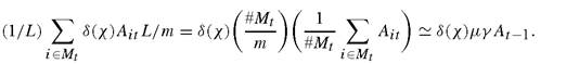
which is also per-capita value-added in the general sector. By similar reasoning, (8) implies that per-capita value added in monopolized intermediate sectors is:

2. Growth increases with the size of innovations, as measured by γ. This result points to the existence of a wedge between private and social innovation incentives. That is, a decrease in size would reduce the cost of innovation in proportion to the ex­pected rents; the research arbitrage equation (9) shows that these two effects cancel each other, leaving the equilibrium level of R&D independent of size. However, Equation (10) shows that the social benefit from R&D, in the form of enhanced growth, is proportional not to γ but to the “incremental size” γ — 1. When γ is close to one it is not socially optimal to spend as much on R&D as when γ is very large, because there is little social benefit; yet a laissez-faire equilibrium would result in the same level of R&D in both cases.

3. Growth is decreasing with the degree of product market competition and/or with the degree of imitation as measured inversely by χ. Thus patent protection (or, more generally, better protection of intellectual property rights), will enhance growth by increasing χ and therefore increasing the potential rewards from in­novation. However, pro-competition policies will tend to discourage innovation and growth by reducing χ and thereby forcing incumbent innovators to charge a lower limit price. Existing historical evidence supports the view that property rights protection is important for sustained long-run growth; however the predic­tion that competition should be unambiguously bad for innovations and growth is questioned by all recent empirical studies, starting with the work of Nickell (1996) and Blundell, Griffith and Van Reenen (1999). In Section 4 we shall argue that the Schumpeterian framework outlined in this section can be extended so as to recon­cile theory and evidence on the effects of entry and competition on innovations, and that it also generates novel predictions regarding these effects which are borne out by empirical tests.

3.