Linking growth to development: convergence clubs

With its emphasis on institutions, the Schumpeterian growth paradigm is not restricted to dealing with advanced countries that perform leading-edge R&D. It can also shed light on why some countries that were initially poor have managed to grow faster than industrialized countries, whereas others have continued to fall further behind.

The history of cross-country income differences exhibits mixed patterns of conver­gence and divergence. The most striking pattern over the long run is the “great diver­gence” - the dramatic widening of the distribution that has taken place since the early 19th Century. Pritchett (1997) estimates that the proportional gap in living standards between the richest and poorest countries grew more than five-fold from 1870 to 1990, and according to the tables in Maddison (2001) the proportional gap between the rich­est group of countries and the poorest^[21] grew from 3 in 1820 to 19 in 1998. But over the second half of the twentieth century this widening seems to have stopped, at least among a large group of nations. In particular, the results of Barro and Sala-i-Martin (1992), Mankiw, Romer and Weil (1992) and Evans (1996) seem to imply that most countries are converging to parallel growth paths.

However, the recent pattern of convergence is not universal. In particular, the gap between the leading countries as a whole and the very poorest countries as a whole has continued to widen. The proportional gap in per-capita income between Mayer- Foulkes’s (2002) richest and poorest convergence groups grew by a factor of 2.6 be­tween 1960 and 1995, and the proportional gap between Maddison’s richest and poorest groups grew by a factor of 1.T5 between 1950 and 1998. Thus as various authors^[22] have observed, the history of income differences since the mid 20th century has been one of “club-convergence”; that is, all rich and most middle-income countries seem to belong to one group, or “convergence club”, with the same long-run growth rate, whereas all other countries seem to have diverse long-run growth rates, all strictly less than that of the convergence club.

The explanation we develop in this section for club convergence follows Howitt (2000), who took the cross-sectoral-spillovers variant of the closed-economy model described in Section 2.3 and allowed the spillovers to cross international as well as intersectoral borders. This international spillover, or “technology transfer”, allows a backward sector in one country to catch up with the current technological frontier whenever it innovates. Because of technology transfer, the further behind the frontier a country is initially, the bigger the average size of its innovations, and therefore the higher its growth rate for a given frequency of innovations. As long as the country con­tinues to innovate at some positive rate, no matter how small, it will eventually grow at the same rate as the leading countries. (Otherwise the gap would continue to rise and therefore the country’s growth rate would continue to rise.) However, countries with poor macroeconomic conditions, legal environment, education system or credit markets will not innovate in equilibrium and therefore they will not benefit from technology transfer, but will instead stagnate.

This model reconciles Schumpeterian theory with the evidence to the effect that all but the poorest countries have parallel long-run growth paths. It implies that the growth rate of any one country depends not on local conditions but on global conditions that impinge on world-wide innovation rates. The same parameters which were shown in Section 2.4 to determine a closed economy’s productivity-growth rate will now de­termine that country’s relative productivity level. What emerges from this exercise is therefore not just a theory of club convergence but also a theory of the world’s growth rate and of the cross-country distribution of productivity.

Before we develop the model we need to address the question of how our framework, in which growth depends on research and development, can be applied to the poorest countries of the world, in which, according to OECD statistics, almost no formal R&D takes place.

3.1. A model of technology transfer ^[23]

^[1] See Arrow (1969) and Evenson and Westphal (1995).

^[1] Cohen and Levinthal (1989) and Griffith, Redding and Van Reenen (2001) have also argued that R&D by the receiving country is a necessary input to technology transfer.

¹² Again we are assuming a time period small enough to ignore the possibility of simultaneous innovations in the same sector.

¹³ A simpler version of the model would just have the frontier productivity grow at an exogenous rate g. The model in this section has the advantage of delivering both an endogenous rate for productivity growth at the frontier and club convergence towards that frontier.

¹⁴ The growth rate (12) expressed as a log difference is approximately the same as the rate (5) of the previous section which was expressed as a proportional increment, because the first-order Taylor-series approximation to ln γ at γ = 1 is (γ - 1). We switch between these two definitions depending on which is more convenient in a given context.

¹⁵ This is not to say that international trade is unimportant for technology transfer. On the contrary, Coe and Helpman (1995), Coe, Helpman and Hoffmaister (1996), Eaton and Kortum (1996) and Savvides and Zachariadis (2005) all provide strong evidence to the effect that international trade plays an important role in the international diffusion of technological progress. For a recent summary of this and other empirical work, see Keller (2002). Eaton and Kortum (2001) provide a simple “semi-endogenous” (see Section 5) growth model in which endogenous innovation interacts with technology transfer and international trade in goods; in their model all countries converge to the same long-run growth rate.

size:

which is also larger the greater the distance to the frontier.

The distance variable d_t evolves according to:

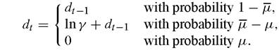
That is, with probability 1 - μ there is no innovation in the sector either globally or in this country, so both domestic productivity and frontier productivity remain unchanged; with probability μ - μ an innovation will occur in this sector but in some other country, in which case domestic productivity remains the same but the proportional gap grows by the factor γ ; and with probability μ an innovation will occur in this sector in this country, in which case the country moves up to the frontier, reducing the gap to zero.

It follows that the expected distance d_t evolves according to:

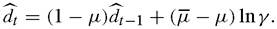
If μ > 0 this is a stable difference equation with a unique rest point. That is, as long as the country continues to perform R&D at a positive constant intensity n its distance to the frontier will stabilize, meaning that its productivity growth rate will converge to that of the global frontier. But if μ — 0 the difference equation has no stable rest point and d_t diverges to infinity. That is, if the country stops innovating it will have a long- run productivity growth rate of zero because innovation is a necessary condition for the country to benefit from technology transfer.

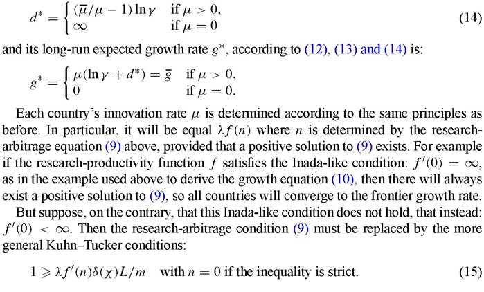
More formally, the country’s long-run expected distance d* is given by:

That is, for an interior solution the expected marginal cost and benefit must be equal, but the only equilibrium will be one with zero R&D if at that point the expected mar­ginal benefit does not exceed the cost. It follows that the country will perform positive R&D if:

but if condition (16) fails then there will be no research: n = 0 and hence no innovations: μ = 0 and no growth: g = 0.

This means that countries will fall into two groups, corresponding to two convergence clubs:

1. Countries with highly productive R&D, as measured by λ, or good educational systems as measured by high λ or high L, or good property right protection as measured by a high χ, will satisfy condition (16), and hence will grow asymptot­ically at the frontier growth rate g.

2. Countries with low R&D productivity, poor educational systems and low prop­erty right protection will fail condition (16) and will not grow at all.

3.2. World growth and distribution

Since the world growth rate g given by (12) depends on each country’s innovation fre­quency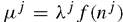, therefore world growth depends on the value for each country

of all the factors described in Section 2.4 that determine μ^j. Thus any improvement in R&D productivity, education or property rights anywhere in the innovating world will raise the growth rate of productivity in all but the stagnating countries.

Moreover, the cross-country distribution of productivity is determined by these same variables. For according to (14) each country’s long-run relative distance to the frontier depends uniquely on its own innovation frequency μ = λf(n). Two countries in which the determinants of innovation analyzed in Section 2.4 are the same will lie the same distance from the frontier in the long run and hence will have the same productivity in the long run. Countries with more productive R&D, better educational systems and stronger property right protection will have higher productivity.

3.3. The role of financial development in convergence

The framework can be further developed by assuming that while the size of innovations increases with the distance to the technological frontier (due to technology transfer), the frequency of innovations depends upon the ratio between the distance to the techno­logical frontier and the current stock of skilled workers. This enriched framework [see Howitt and Mayer-Foulkes (2002)] can explain not only why some countries converge while other countries stagnate but also why different countries may display positive yet divergent growth patterns in the long-run. Benhabib and Spiegel (2002) develop a sim­ilar account of divergence and show the importance of human capital in the process. The rest of this section presents a summary of the related model of Aghion, Howitt, and Mayer-Foulkes (2004) (AHM) and discusses their empirical results showing the importance of financial development in the convergence process.

Suppose that the world is as portrayed in the previous sections, but that research aimed at making an innovation in t must be done at period t — 1. If we assume perfectly functioning financial markets then nothing much happens to the model except that the research arbitrage condition (9) has a discount factor β on the right-hand side to reflect the fact that the expected returns to R&D occur one period later than the expenditure.^[24] But when credit markets are imperfect, AHM show that an entrepreneur may face a bor­rowing constraint that limits her investment to a fixed multiple of her accumulated net wealth. In their model the multiple comes from the possibility that the borrower can, at a cost that is proportional to the size of her investment, decide to defraud her creditors by making arrangements to hide the proceeds of the R&D project in the event of success.^[25] They also assume a two-period overlapping-generations structure in which the accumu­lated net wealth of an entrepreneur is her current wage income, and in which there is just one entrepreneur per sector in each country. This means that the further behind the fron­tier the country falls the less will any entrepreneur be able to invest in R&D relative to what is needed to maintain any given frequency of innovation. What happens in the long run to the country’s growth rate depends upon the interaction between this disadvantage of backwardness, which reduces the frequency of innovations, and the above-described advantage of backwardness, which increases the size of innovations. The lower the cost of defrauding a creditor the more likely it is that the disadvantage of backwardness will be the dominant force, preventing the country from converging to the frontier growth rate even in the long run. Generally speaking, the greater the degree of financial devel­opment of a country the more effective are the institutions and laws that make it difficult to defraud a creditor. Hence the link between financial development and the likelihood that a country will converge to the frontier growth rate.

The following simplified account of AHM shows in more detail how this link be­tween financial development and convergence works. Suppose that entrepreneurs have no source of income other than what they can earn from innovating. Then they must borrow the entire cost of any R&D project. Because there are constant returns to the R&D technology,^[26] therefore in equilibrium that cost will equal the expected benefit, discounted back to today:

This is also the expected discounted benefit to a borrower from paying a cost cN_t today that would enable her to default in the event that the R&D project is successful. (There is no benefit if the project fails to produce an innovation because in that case the en­trepreneur cannot pay anything to the creditor even if she has decided to be honest and therefore has not paid the cost cN_t.) The entrepreneur will choose to he honest if the cost at least as great as the benefit; that is, if:

Otherwise she will default on any loan.

Suppose that βλδ(χ)L∕m > 1/f '(0). This is the condition (16) above for positive growth, modified to take discounting into account. It follows that in any country where the incentive-compatibility constraint (17) holds then innovation will proceed as de­scribed in the previous section, and the country will converge to the frontier growth rate. But in any country where the cost of defrauding a creditor is less than unity no R&D will take place because creditors would rationally expect to be defrauded of any possible return from lending to an entrepreneur. Therefore convergence to the frontier growth rate will occur only in countries with a level of financial development that is high enough to put the cost of fraud at or above the limit of unity imposed by (17).

AHM test this effect of financial development on convergence by running the follow­ing cross-country growth regression:

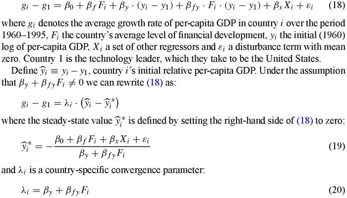
that depends on financial development.

A country can converge to the frontier growth rate if and only if the growth rate of its relative per-capita GDP depends negatively on the initial value ^y_i; that is if and only if the convergence parameter λ_i is negative. Thus the likelihood of convergence will increase with financial development, as implied by the above theory, if and only if:

The results of running this regression using a sample of 71 countries are shown in Ta­ble 1, which indicates that the interaction coefficient βf_y is indeed significantly negative for a variety of different measures of financial development and a variety of different conditioning sets X. The estimation is by instrumental variables, using a country’s legal origins,^[27] and its legal origins interacted with the initial GDP gap (y_i - y₁) as instru­ments for F_i and F_i (y_i - y₁). The data, estimation methods and choice of conditioning sets X are all take directly from Levine, Loayza and Beck (2000) who found a strongly positive and robust effect of financial intermediation on short-run growth in a regres­sion identical to (18) but without the crucial interaction term F_i(y_i - y₁) that allows convergence to depend upon the level of financial development.

AHM shown that the results of Table 1 are surprisingly robust to different estimation techniques, to discarding outliers, and to including possible interaction effects between the initial GDP gap and other right-hand-side variables.

3.1. Concludingremark

Thus we see how Schumpeterian growth theory and the quality improvement model can naturally explain club convergence patterns, the so-called twin peaks pointed out by Quah (1996). The Schumpeterian growth framework can deliver an explanation for cross-country differences in growth rates and/or in convergence patterns based upon in­stitutional considerations. No one can deny that such considerations are close to what development economists have been concerned with. However, some may argue that the quality improvement paradigm, and new growth theories in general, remain of lit­tle help for development policy, that they merely formalize platitudes regarding the growth-enhancing nature of good property right protection, sound education systems, stable macroeconomy, without regard to specifics such as a country’s current stage of development. In Sections 4 and 6 we will argue on the contrary that the Schumpeterian growth paradigm can be used to understand (i) why liberalization policies (in particular an increase in product market competition) should affect productivity growth differently in sectors or countries at different stages of technological development as measured by the distance variable d; and (ii) why the organizations or institutions that maximize growth, or that are actually chosen by societies, also vary with distance to the frontier.

4.