Calibrating the impact of the misallocation of capital
In this long list of potentially distorting factors there are some, like government failures or credit market failures, that most people find a priori plausible, and others, such as intra-family inefficiencies or learning externalities, that are more contentious, and yet others, like the behavioral factors, that have not yet been widely studied.
However, even where the prima facie evidence is the strongest, we cannot automatically conclude that the particular distortion has resulted in a significant loss in productivity.To get a sense of the potential productivity loss, we return to the Indo-U.S. comparison. Taking as given the stock of capital in India and the U.S. today, any of the multiple distortions listed above could have affected productivity in two different ways: First, there may be across-the-board inefficiency, because everyone could have chosen the wrong technology or the wrong product mix. Second, capital may be misallocated across firms: There may be differences in productivity across firms, either because of differences in scale, or because of differences in technology or because some entrepreneurs are more skilled than others, and the distribution of capital across these firms may be sub-optimal, in the sense that the most productive firms are too small.
32
Here we have chosen to emphasize this latter source of inefficiency, motivated in part by the evidence, discussed above, that tells us that there are enormous differences in productivity across firms. We take no stance on how such an inefficient allocation of capital came about, nor on why the firms do not make the right choices, either of scale or technologies. Lack of access to credit is, of course, a potential explanation for both, but it could equally be explained by lack of insurance, the fear of confiscation by the government, or the gap between real and perceived returns.
The goal of this section is to set-up and calibrate a simple model, to investigate whether the misallocation of capital across firms within a country can explain the aggregate puzzles we started from: the low output-per-worker in developing countries, given the level of capital, and the low marginal product of capital, given the output- per-worker. We do not claim that we necessarily have the right explanation; there are simply too many degrees of freedom in this kind of exercise. Nevertheless we feel that the exercise has some value, not least because it gives us some reason to believe that we have not been entirely misguided in emphasizing the role of misallocation. Moreover, as we will see, it does rule on some kinds of misallocation stories in favor of others.
We begin with a model where the misallocation only affects the scale of production, because all the firms share the same technology. Scale obviously does not matter where there are constant returns to scale, so we need to turn to a model where there are diminishing returns at the firm level.[301] We will show that, with realistic assumptions about the relative firm size in India and the U.S., this model cannot go very far in explaining the aggregate facts. We then turn to a model where a better technology can be purchased for a fixed cost. We show that this model, coupled with the misallocation of capital, will help generate the aggregate facts, with realistic assumptions about the distribution of firm sizes.
5.1. A model with diminishing returns
• Model set-up
Consider a model where there is a single technology that exhibits diminishing returns at the firm level, say, Y = ALγ Kα, with γ < 1 - α. Also, we will assume that the economy has a fixed number of firms: Without that assumption, everyone will set up multiple minuscule firms, thereby eliminating the diminishing returns effect. To justify this we make the standard assumption that the economy has a fixed number of entrepreneurs and each firm needs an entrepreneur.
Under these assumptions every firm would invest the same amount when markets function perfectly, but when different firms are of different sizes, the marginal product would vary across the firms and efficiency would suffer. The question is whether these effects are large enough to help us explain what we see in the data. Given that we are
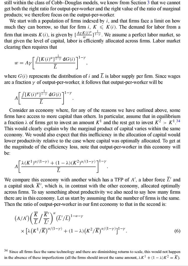
Table 3
Distribution of firm size (Annual Survey of Industry, 2000)
| 95-5 ratio | median-5 ratio | mean-5 ratio | 5th percentile | |
| Manufacture of pasteurized milk | 1007 | 95 | 216 | 61466 |
| Flour milling | 786 | 150 | 285 | 29899 |
| Rice milling | 1392 | 90 | 620 | 5681 |
| Cotton spinning | 22300 | 440 | 5423 | 12870 |
| Cotton weaving | 3093 | 31 | 1292 | 14159 |
| Textile garment manufacture | 1581 | 104 | 410 | 22461 |
| Curing raw hides and skins | 235 | 10 | 53 | 37075 |
| Manufacture of footwear | 2639 | 122 | 683 | 21825 |
| Manufacture of car parts | 1700 | 29 | 504 | 84103 |
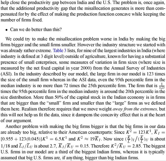
Finally note that in our model, the ratio of the 95th percentile firm to the 5th percentile firm in the median industry is approximately 1600 : 1.35 Giventheproductionfunction, we know that the marginal return on capital in the two firms should differ by a factor of 16001/2 = 40 : 1.
If the biggest firms pay about 9% for their capital, the smaller firms must have a marginal product that exceeds 360%, which seems implausible. Making the gap between small and large firms even larger would clearly exacerbate this problem.Another possible way to augment the productivity gap is to give up the assumption that the two economies have same number of firms. Suppose the U.S. had λ > 1 times as many firms as India: Then the labor productivity ratio computed above would have to be divided by λ1~α~r. If λ were equal to 32, the ratio of labor productivity in India to that in the U.S. would be 9%, which is what we find in the data.
Of course, increasing the number of the firms in the U.S. will tend to make the average firm in the U.S. smaller: Even with the same number of firms in the two countries, the fact that the biggest firms in India have about 18 times the average capital stock means that they are about 3 times the size of U.S. firms, which seems implausible. If there are 32 times as many firms in the U.S., the average U.S. firm would be about a 1∕100th of the biggest Indian firm, close to 25% in the Indian size distribution. This seems entirely counterfactual.
• Taking stock
To sum up, moving to this more sophisticated model does not help us fit the macro facts better. It obviously does suggest a simple theory of the cross-sectional variation in returns to capital, which is entirely absent from the model with constant returns, but ends up throwing up a number of other problems that a theory of this type will need to deal with. In particular, a successful explanation has to be consistent with the fact that the firm size distribution in India has a large part of its weight near the mean/median; that even the biggest Indian firms are not larger than the bigger U.S. firms in the same industry; and that the marginal product of capital in the average small Indian firm, while large (even 100%) is probably not 300% or more.
The next section introduces an alternative model where firms differ both in scale and in technology, but still retains the assumption that there is no inherent difference between these alternative investors.
5.2. Amodelwithfixedcosts
• Model set up
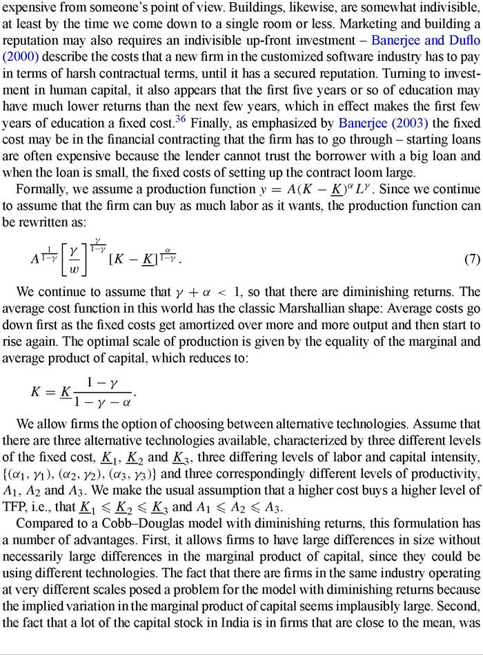
Consider a world where setting up requires a fixed start-up cost in addition to an entrepreneur, but once these are in place, capital and labor get combined as in a standard Cobb-Douglas with diminishing returns. This fixed cost could come from many sources: Machines come in certain discrete sizes and even the smallest machine may be
35 The median industry is the Textile Garment Manufacturing industry.
[1] All the estimates (14) we could find of Mincerian returns at different levels of education suggest that, in developing countries, the marginal benefit of a year of education increases with the level of education (in the U.S., it appears to be very flat). Schultz (2004) finds the same result in his study of six African countries.
a problem when we had global diminishing returns, because with diminishing returns, firms close to the mean are at the optimal scale. In our present model, the right scale for Indian firms is actually much bigger than the mean. A part of the inefficiency comes precisely from the fact that there are many firms that are concentrated near the mean. Third, as noted above, this model generates a unique optimal scale of production, which would provide a reason why the biggest (and most productive) Indian and U.S. firms could be more or less the same size. Fourth, because efficient firms tend to be quite large, it is easy to see why India, with its multitude of firms that are too small, will be inefficient relative to the U.S., where all firms are at the right scale. Fifth, the fact that production requires a fixed cost helps explain why, despite the diminishing returns from technology, we do not see people setting up a very large number of very small firms, thereby completely eliminating the diminishing returns effect.
In this case, we can let the number of firms be determined by what people are willing to invest, in combination with what we know about the fixed costs (actually as noted below, we cheat slightly on this point, but only because it simplifies the calculations). Sixth, the fact that we allow the number of firms to be determined endogenously means that there are less overall diminishing returns. When we compare the U.S. and India, this helps explain why the productivity gap is so large and why interest rates are not lower in the U.S. Finally making this assumption alters the nature of the link between the marginal product of capital and its average product. With a Cobb-Douglas, the ratio of the average product is always proportional to the marginal product. Here, the average product starts lower than the marginal product but grows faster and eventually becomes larger than the marginal product. In other words, as firm size goes up the ratio of the marginal product of capital to its average product goes down, at least initially. This would suggest that the ratio of the average products of capital in India and the U.S. should be less than the ratio of the marginal products, and indeed we find that while output-per-worker is 11 times larger in the U.S., capital-per-worker is 18 times as large, implying an average product ratio of about 1.6 : 1, as against the 2.5 : 1 ratio of marginal products delivered by the standard Cobb-Douglas model. This is clearly an a priori advantage of this formulation, since, as we noted in Section 3, the proportionality between the average product and the marginal product prevents any model based on a Cobb-Douglas production function to fit these facts.Interestingly, this model brings together elements - market imperfections and some increasing returns - that are also being invoked by recent work in new growth theory [Aghion et al. (2004), for example] for the same purpose, namely to explain the lack of convergence. However, the increasing returns and the credit constraints here are at the level of the firm, whereas in the aggregative growth literature they are at the level of the economy. Indeed, if there is no misallocation and no lack of people to start new firms, the aggregate production function generated by our economy exhibits constant returns in labor and capital: Indeed it has exactly the form that Lucas started with - Y = AKαL1-α.
In order to impose restrictions on the parameters of the model, we make use of the industry data described in Table 3. We describe the representative Indian industry by a 3-point distribution of firms sizes, with fractions λ1, λ2, and λ3 at K1, K2 and K3. The first group of firms is made of the bottom 10% of the distribution of firms, and we assigned to them the size of the firm at the 5th percentile of the actual size distribution in the data. Likewise, we assume that the top 10% of all firms are in the group of “large firm”, and that their size is that of the firm at the 95th percentile of the firm size distribution.[302] The rest we assign to the middle category, whose size we set at the mean for the distribution. We assume that the largest firm is 1,600 times as big as the smallest firm, which is roughly the median value of these ratios across these nine industries in our data.
These parameter values imply that the mean firm size in the industry will be 800 times as large as the 5th percentile firm, which is higher than the mean in the median industry in our data (500 times), but well within the existing range in the data. Once again we are interested in the within-economy variation in returns to capital. We therefore assume, as before, that the small firms have a marginal product of 100% while the medium sized firms have a marginal product of just 9%.
The more unorthodox assumption is that the large firms also have a marginal product of 100%. While clearly somewhat artificial, this is meant to capture the idea that the best technology is expensive and only the biggest firms in India can afford to be at the cutting edge, an idea that is very much in the spirit of the McKinsey Global Institute’s study of a number of specific Indian industries. However, they are still relatively small and therefore the marginal returns on an extra dollar of investment are very high. The rest of the firms use cheaper (i.e., lower K) but less effective technologies. In particular, the small firms are simply too small (which explains their high marginal product), and the middle category consists of firms that have exhausted the potential of the mediocre technology that they can afford but are too small to make use of the ideal technology.
How plausible is our assumption about industry structure? The average capital stock of the 95th percentile firms in the median industry was Rs. 36 million, which puts them at a size just above the category of firms that are the focus of Banerjee and Duflo (2004). The point of that paper was that a subset of these firms (the firms that attracted the extra credit after the policy change) had marginal returns on capital of close to 100%. Therefore it is not absurd to assume that the large firms in our model economy have very high returns. Once we accept the idea that some large firms are very productive, given that the average marginal product is probably close to 22%, it is obviously very likely that there are many smaller firms that have a lower marginal product than the largest firms. Indeed, when we calculate the average marginal product based on our assumptions, under the premise that the marginal dollar is distributed across the three size categories in the ratio of their share in the capital stock, the average marginal product turns out to be about 27%.
Even with this long list of assumptions, we do not have enough information to compute output-per-worker in our model economy - there are several remaining degrees
[1] This is where we cheat, since with decreasing returns to scale, there could again be an infinity of very small firms, so that all the firms should be in the small group. We can prevent that if we assume that the smallest feasible firm size is actually ε greater than zero, and only a certain number of entrepreneurs are able (or willing) to invest at least ε.
attract all those in India who have nowhere better to go. While there are only a few such industries, they are enormous, and quite unlike the rest of the industries: Among the industries listed in the table above, cotton spinning is probably most like what one of these industries looks like, and it is apparent that it is quite different from the rest - there are many more tiny firms.
However this is not a problem for what we are doing here. Starting with the Indian firm size distribution assumed in the above exercise, we could simply add many more of the smallest firms to the Indian firms size distribution, until we get to the point where India has the same number of firms as the U.S. Since we have increased the number of firms in India by 3∣ times while keeping the number of large firms (firms with 1,600 units of capital) constant, the share of these firms goes down to 3% (from 10%). These two versions of the Indian economy are reasonably similar, because the smallest firms do not add up to a large amount of capital, but it is obvious that this economy will be less productive than the previous one (since inefficient small firms will have a larger share of total capital), and hence we will actually get somewhat closer to the 11 : 1 productivity ratio that we were shooting for.
• Why doesn’t capital flow to India?
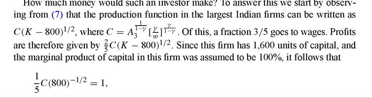
Finally we subject this model to an additional test: The fact that in our model there are firms in India with returns in the neighborhood of 100% would suggest that there are many unexploited opportunities. We have already argued that there are many reasons why a U.S. bank could not just lend to an Indian firm, and thereby benefit from these opportunities. Nor is it easy for an American to borrow money in the U.S. and set up a firm in India: Once he is in India he may be beyond the reach of U.S. law and for that reason alone, lenders will shy away from him. What is much more plausible, however, is that a U.S. entrepreneur moves to India to invest his money in these opportunities. The question is why this does not happen more often.
There are some obvious answers to this question: If the reason why these opportunities have not already been taken is the lack of secure property rights in India, there is no reason why foreigners would be particularly keen to invest in India. On the other hand, if the problem is that Indians do not have the capital or that they fear the risk exposure or that they are simply unaware of the opportunity, to take some plausible alternatives, a well-diversified wealthy U.S. investor may well be attracted to move to India and start a firm.
or
C = 141.42.
The opportunity cost of capital for a U.S. investor is 9%. The optimal investment in this Indian firm for a U.S. investor who can invest as much as he wants will be given by the solution to

This tell us that the optimal investment is K = 99564. The total after-wage income generated by the firm is (0.4)(141.42)(99564 — 800)1/2 = 17777. This is in units of the smallest firm. We know that the biggest firms in our model are 1,600 times as large as the smallest firms and from the table above, such firms have Rs. 36 million worth of capital in the median industry. The smallest firm therefore has Rs. 22,500 worth of capital, which implies that the U.S. investor will earn 17777(22500) = Rs. 400 million on his investment of (99564)(22500) = Rs. 2.24 billion. This is a net gain of about Rs. 200 million, or about 4 million dollars.
Is this a large enough gain to tempt someone to leave his home and family and settle in India? For someone with an average income, obviously. But no one with an average income has 50 million dollars of his own that he is willing to put into a single project in India. Anyone who is willing to do it has to be very rich indeed - he must have $50 million several times over. How many people are so wealthy that they are willing to give up their life in the U.S. for an extra $4 million per year?
In other words, while the model developed in this section generates very large productivity losses, it does not offer any one person the possibility of arbitraging these unexploited opportunities to become enormously rich. This is because diminishing returns set in quite fast.
5.2.1. Taking stock
We started by describing some of the major puzzles left unanswered by the neo-classical model, and in particular the productivity gap between rich and poor countries. The coexistence of high and low returns to investment opportunities, together with the low average marginal product of capital, suggested that some of the answer might lie in the misallocation of capital. The microeconomic evidence indeed suggests that there are some sources of misallocation of capital, including credit constraints, institutional failures, and others. In this section, we have seen that, combined with multiple technological options and a fixed cost of upgrading to better technologies, a model based on misallocation of capital does quite well in terms of explaining the productivity gap. The value of the marginal productivity of capital in the U.S. predicted by this model is only marginally too high, and the degree of variation in the marginal product of capital within a single economy that the model requires is not implausibly large.
Of course the model does make unrealistic assumptions - there is, for example, surely some amount of inefficiency in the U.S., and some U.S. firms are surely more productive than others. On the other hand, we have also ignored many reasons why Indian firms may be less efficient than they are in our model. For example, our current model assumes that only 10% of the firms, who use less than 1% of the capital stock and produce less than 1% of the output, use the least efficient technology whereas the MGI report on the apparel sector tells us that almost 55% of the output of the sector is produced by tailors who still use primitive technology. We also assumed that 10% of Indian firms are as productive as the best U.S. firms. Clearly that fraction could be smaller.
We also assumed that everyone is equally competent. In the real world, imperfect credit markets, for example, drive down the opportunity cost of capital and this encourages incompetent producers to stay in business. In the model, we assume that all large firms earn high returns but in reality there are probably some large firms that have much lower productivity (anywhere down to 9% per year would be consistent with our model). This too will drive down productivity. In a recent paper, Caselli and Gennaioli (2002) try to calibrate the impact of this factor in the context of a dynamic model with credit constraints. They show that in steady state this can generate productivity losses of 20% or so. We will argue in the next section that this severely understates the potential productivity gap starting from an arbitrary allocation of capital.