Comparison Between Alternative Seasonal Adjustments

When we deal with consumer data in general, we need to make seasonal adjustments. We used two main alternative methods of adjustments on our data. The first

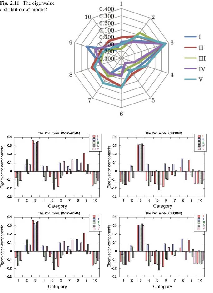
Fig.

2.12 Comparison between X-12-ARIMA and DECOMP

Table 2.4 Mode 1 (eigenvalue A₁ = 4.24)

	I	II	III	IV	V
1 Food	0.288	0.275	0.281	0.283	0.335
2 Housing	-0.069	-0.070	-0.024	0.034	0.018
3 Fuel, light and water charges	0.088	0.193	0.189	0.161	0.128
4 Furniture and household utensils	0.137	0.091	0.067	0.153	0.030
5 Clothing and footwear	0.086	0.264	0.058	0.161	0.176
6 Medical care	0.049	-0.059	0.115	0.109	-0.032
7 Transportation and communication	0.098	0.083	-0.056	0.169	0.005
8 Education	0.005	-0.088	0.035	-0.160	0.071
9 Culture and recreation	0.141	0.171	0.071	0.043	0.171
10 Other	-0.056	0.096	0.094	-0.019	0.122

Note: The data used are from Jan 2000 to Feb 2012

Table 2.5 Mode 2 (eigenvalues A₂ = 3.54)

bgcolor=white>-0.026

	I	II	III	IV	V
1 Food	-0.073	-0.009	-0.171	-0.104	-0.108
2 Housing	0.002	0.076	0.139	-0.023	0.079
3 Fuel, light and water charges	0.362	0.327	0.310	0.342	0.355
4 Furniture and household utensils	0.000	0.065	-0.058	-0.106	0.061
5 Clothing and footwear	-0.064	-0.027	-0.133	-0.210	-0.081
6 Medical care	-0.175	0.102	-0.073	-0.046	0.121
7 Transportation and communication	-0.025	0.059	0.021	-0.028	0.137
8 Education	0.001	0.143	0.012	0.010	0.101
9 Culture and recreation	0.217	0.010	-0.028	0.089
10 Other	-0.162	-0.002	-0.141	-0.072	-0.111

Note: The data used are from Jan 2000 to Feb 2012

was X-12-ARIMA,^[35] developed and used by the U.S. Census Bureau.

It is also a standard seasonal adjustment method used by the Statistics Bureau in Japan. The X- 12-ARIMA program draws on experimental evidence, with a number of degrees of freedom for users to optimize the procedure. However, we allowed the program to determine a best-fit model by itself. The second was DECOMP,^[36] developed by the Institute of Statistical Mathematics, Japan. The basis of the two is quite different. In our application, surprisingly, the derived results are very similar for the principal components, and show that the largest eigenvalue is dominated by FOOD, and the second by FUEL, LIGHT, & WATER. In other words, the first component is constructed by the explanatory category dominated by FOOD, and the second by the category dominated by FUEL, LIGHT & WATER. These results are shown diagrammatically in Fig. 2.12.

2.4

<< | >>

↑

Source: Aruka Y.. Evolutionary Foundations of Economic Science: How Can Scientists Study Evolving Economic Doctrines from the Last Centuries? Springer Japan,2015. — 234 p.. 2015

More economic literature on Economics.Studio

Comparison Between Alternative Seasonal Adjustments

More on the topic Comparison Between Alternative Seasonal Adjustments: