An Empirical Study Using Input-Output Tables
The inter-industrial input-output table is readily available to provide empirical information. This table has common classification rules, so the number of industries is usually fixed for particular periods, though some revisions of classifications are intermittently incorporated, and groupings may therefore change periodically.
The Input-Output Tables in Japan, released every 5 years since 1955, are the most important statistics for the revision of standards and extended estimation of GDP for the calculation of the National Accounts by the Japanese Cabinet Office. The tables are produced by several Government agencies.[45]
The table is based on Basic Sector Tables, with 520 rows x 407 columns. The tables are of various sizes ranging from 13 to 34 and 108 to 190-sector classifications. We used 13 or 34-sector tables for convenience, covering the years 1995, 2000, and 2005. There was no 34-sector table in 2000, as it only has 32 sectors, because the items “14 Information and communication electronics equipment” and “15 Electronic components” were not explicitly given as formal sectors. We can regard these items as emerging links between 2000 and 2005. In other words, the input-output system structurally evolved in this time. The items of sector classification are shown in Table 3.3.
3.4.1 The First Step Towards Empirical Input-Output Analysis
We have argued an elementary analysis in a general case of a joint-productive system, which permits the system to produce a set of multiple outputs in a single process of production. However, the empirical data such as the input-output table
Table 3.3 Sector classifications
| 13 sectors in 1995; 2000; 2005 | 32 sectors in 2000 | 34 sectors in 2005 |
| 01 Agriculture, forestry and fishery | ||
| 02 Mining | ||
| 03 Manufacturing | ||
| 04 Construction | ||
| 05 Electric power, gas and water supply | ||
| 06 Commerce | ||
| 07 Finance and insurance | ||
| 08 Real estate | ||
| 09 Transport | ||
| 10 Communication and broadcasting | ||
| 11 Public administration | ||
| 12 Services | ||
| 13 Other activities | 01 Agriculture, forestry and fishery | 01 Agriculture, forestry and fishery |
| 02 Mining | 02 Mining | |
| 03 Beverages and foods | 03 Beverages and foods | |
| 04 Textile products | 04 Textile products | |
| 05 Pulp, paper and wooden products | 05 Pulp, paper and wooden products | |
| 06 Chemical products | 06 Chemical products | |
| 07 Petroleum and coal products | 07 Petroleum and coal products | |
| 08 Ceramic, stone and clay products | 08 Ceramic, stone and clay products | |
| 09 Iron and steel | 09 Iron and steel | |
| 10 Non-ferrous metals | 10 Non-ferrous metals | |
| 11 Metal products | 11 Metal products | |
| 12 General machinery | 12 General machinery | |
| 13 Electrical machinery | 13 Electrical machinery | |
| N/A | 14 Information and communication electronics equipment | |
| N/A | 15 Electronic components | |
| 14 Transportation equipment | 16 Transportation equipment |
(continued)
Table 3.3 (continued)
| 13 sectors in 1995; 2000; 2005 | 32 sectors in 2000 | 34 sectors in 2005 |
| 15 Precision instruments | 17 Precision instruments | |
| 16 Miscellaneous manufacturing products | 18 Miscellaneous manufacturing products | |
| 17 Construction | 19 Construction | |
| 18 Electricity, gas and heat supply | 20 Electricity, gas and heat supply | |
| 19 Water supply and waste disposal business | 21 Water supply and waste disposal business | |
| 20 Commerce | 22 Commerce | |
| 21 Finance and insurance | 23 Finance and insurance | |
| 22 Real estate | 24 Real estate | |
| 23 Transport | 25 Transport | |
| 24 Information and communications | 26 Information and communications | |
| 25 Public administration | 27 Public administration | |
| 26 Education and research | 28 Education and research | |
| 27 Medical service, health, social security and nursing care | 29 Medical service, health, social security and nursing care | |
| 28 Other public services | 30 Other public services | |
| 29 Business services | 31 Business services | |
| 30 Personal services | 32 Personal services | |
| 31 Office supplies | 33 Office supplies | |
| 32 Other activities | 34 Other activities |
Data source: Input-Output Tables for Japan, published by the Statistics Bureau, Director-General for Policy Planning (Statistical Standards), and Statistical Research and Training Institute.
See http://www.stat.go.jp/english/data/io/index.htmusing industrial sectors require the special but practical idea of a single output from a single process of production. This peculiarity of the input-output analysis therefore limits our tool set for inter-industrial network analysis.
3.4.1.1 The Closeness Centrality
In Sect. 3.2, we mentioned that there is often an egalitarian eigenvector centrality in the input-output table. We therefore employ the idea of closeness centrality to characterize the inter-industrial network. The definition of closeness centrality (see
Freeman 1978/1979; Opsahl et al. 2010; Wasserman and Faust 1994) is:
Here i is the focal node and j is another node in the targeted network, while dij∙ is the shortest distance between these two nodes.[46]
3.4.1.2 The Historical Transitions in the 13-Sector Classification
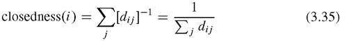
Although the definitions have not remained entirely constant over time, the 13-sector classification is consistent enough over the last three periods, 1995,2000, and 2005. We look first at the transition between the three periods. There is a fixed set of graph communities like categories {1,3,4} and {2, 5, 9} across all three periods. However, components {6,7, 8,10,11,12,13} have separated into subsets. We can show the evolution of the weighted adjacency graph highlighted by the closeness centrality across the period as Figs. 3.10, 3.11, and 3.12.
We can also summarize the transitions among the graph communities in table form, in Table 3.4.
3.4.1.3 An Application to a More Expanded Case: 32 to 34-Sector Classification
We can apply the same analysis of closeness centrality and graph communities to the 32-sector case in 2000 (Fig. 3.13) and the 34-sector case in 2005, producing diagrams of the highlighted graph of the weighted adjacent matrix, and the transitions among the graph communities.
See Fig. 3.14 and Table 3.5.The operation to add two nodes, 14 and 15, does not imply real change for the whole system of production, because the actual production network has not changed at all after this statistical procedure. The added nodes require a nominal change of the existing wiring network, with almost immediate replacement of link attachments. We may therefore interpret these added nodes alongside the missing nodes in the existing inter-industrial network. By renormalization, these two missing nodes have been revealed. If the added nodes are missing and to be renewed, i.e., disconnected, the system under observation could be a closed system, and we may regard a newly emerging community as a newly wired set of links, irrespective of the real change in the whole value.[47]
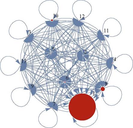
Fig. 3.10 The highlighted graph of the weighted adjacent matrix in 1995
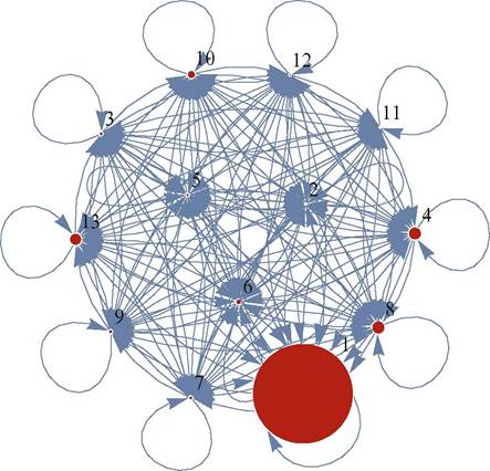
Fig. 3.11 The highlighted graph of the weighted adjacent matrix in 2000
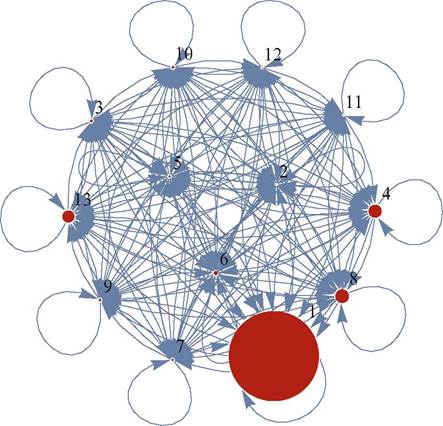
Fig. 3.12 The highlighted graph of the weighted adjacent matrix in 2005
Table 3.4 Transitions among the graph communities in the 13-sector case
| Year | Graph communities |
| 1995 | {{6, 7, 8, 10, 11, 12, 13}, {1, 3, 4}, {2, 5, 9}} |
| 2000 | {{7, 8, 11, 13}, {1, 3, 4}, {2, 5, 9}, {6, 10, 12}} |
| 2005 | {{6, 8, 10, 12}, {1, 3, 4}, {2, 5, 9}, {7, 11, 13}} |
It is immediately seen that the community {2, 22, 23, 24, 25, 26, 28, 30, 31, 32, 34}, by renaming previous items, has reduced itself to a smaller sub-community :{21, 23, 24, 26, 27, 30, 31, 34}.
On the other hand, an emerging community {13, 14, 15, 17, 28} around the two nodes 14 and 15 has absorbed 13, 17, and 28, which previously belonged elsewhere. We have successfully traced a new community formation in the inter-industrial network.Finally, in Figs. 3.15 and 3.16, we show a set of graphical presentations corresponding to Table 3.3.
equivalence between a Polya urn process and a renewal of the network spanned by a closed number of links. Taking into account that a finite set of productive processes on the input-output table is given, and using Ohkubo’s rule, we can show a renewal process of the network of production under the preferential attachment within the closed set of links. Here we regard a replacement of link attachment as a replacement of a productive process.
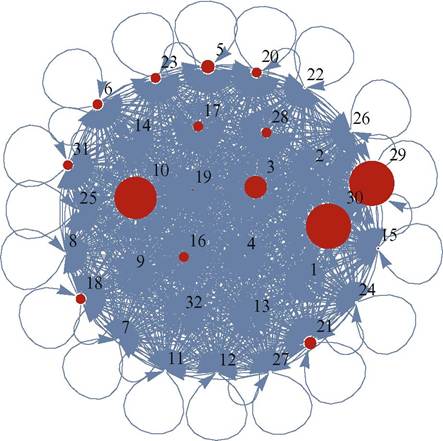
Fig. 3.13 The highlighted graph of the weighted adjacent matrix in 2000
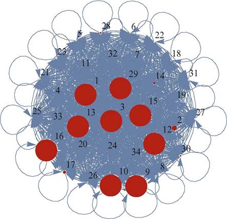
Fig. 3.14 The highlighted graph of the weighted adjacent matrix in 2005
Table 3.5 Transitions among the graph communities in the 32/34-sector case
| Year | Graph communities |
| 2000 | {2, 20, 21, 22, 23, 24, 26, 28, 29, 30, 32}, {3, 4, 5, 6, 16, 19, 27, 31}, {8, 9, 10, 11, 17}, {12, 13, 14, 15, 25}, {1, 7, 18} |
| 2000* | {2, 22, 23, 24, 25, 26, 28, 30, 31, 32, 34}, {3, 4, 5, 6, 18, 21, 29, 33}, {8, 9, 10, 11, 19}, {12, 13, 16, 17, 27}, {1, 7, 20} |
| 2005 | {21, 23, 24, 26, 27, 30, 31, 34}, {2, 7, 8, 20, 25}, {13, 14, 15, 17, 28}, {5, 18, 22, 33},{9, 11, 12, 19}, {1, 3, 32}, {4, 6, 29}, {10}, {16} |
* Re-numbers to reflect classification in 2005
3.4.2 A Further Consideration for Empirical Studies
of the Inter-Industrial Network
In the input-output table, new links in the input-output analysis will occur when a new classification rule is employed, as we have seen by comparing the 32-sector classification in 2000 and the 34-sector classification 5 years later.
As long as we are focused on the input-output analysis, therefore, it is difficult for us to analyze a true process of newly created links, i.e., a truly innovative process. In our empirical framework, we are forced to use an indirect approach to detect innovation and its effect on the network using the inter-industrial input-output tables.We now mention two considerations for future work.
3.4.2.1 External Links from Export Industries
In this chapter, we have not explicitly introduced the price system, so we have not considered the causes of technological changes driven by the price system. We can temporarily examine some of the effects from the demand side through export industries. The inter-industrial network analysis compactly summarizes the production inducement coefficient due to export from each industry, and the effects caused by the export activities. Roughly speaking, the average coefficient of this during the last decade is estimated as 2.[48] Each unit of export can contribute about twice its export size to its activity level. The change in exports over different industries will induce a new wiring set of links independently, irrespective of domestic demand links. The export industry is therefore an important demand link that contributes directly to the domestic inter-industrial network. The next step is to introduce the components of export directly matched to the domestic supply network.
Fig. 3.15 The set of re-combinatorial wiring communities of the inter-industrial network in 2000
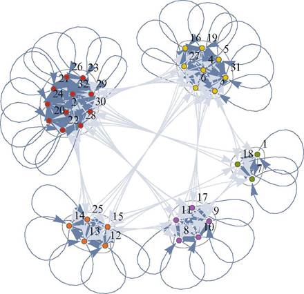
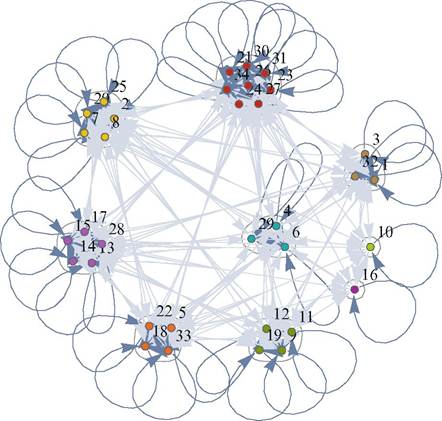
Fig. 3.16 The set of re-combinatorial wiring communities of the inter-industrial network in 2005
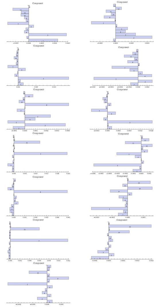
Fig. 3.17 The component distributions of eigen-sectors in the 13-sector table in 2005
3.4.2.2 The Trade-Off Relationships Between Industrial Components or Communities
Recently, it has been discernible that financial activities may invalidate the activities of other real industrial sectors.
By applying covariance analysis to the input coefficient matrix of the input-output table, we can characterize each eigen-mode by its principal component with the largest value.[49] If the principal component is the seventh element, the eigen-mode may be dominated by the finance industry; that is, the seventh in Table 3.3. We can then find opposite signs in each eigenmode. In such a case, the dominant component may react in the opposite direction to other associated industries with opposing signs. These observations must be helpful to provide a rough profile of the swap or trade-off between different industrial activities.Figure 3.17 shows the component distributions in each eigen-sector. This type of analysis will also contribute to finding a potential linkage to change the development of the inter-industrial network.
The network analysis has become popular in this century. The analysis of hierarchically nested structures will be developing. As the network analysis advances, the traditional subjects of economics will be recovered by employing a newly emerging network analysis. In fact, some of classical economists virtually shared with the same focus as the modern network analysis.