An Essential Characteristic of the Joint-Production System
An input-output relationship is a process i producing a single independent unit 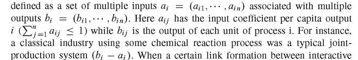 processes has been created, a spanned system of production among the links may not necessarily guarantee the coincidence of the number of processes (input) with the number of commodities (output) in view of a given technology.
3.3.1 An Acyclic Network of Production
The idea of an acyclic network is much broader than function. The function merely indicates a single outflow, even with multiple inflows. It will easily be seen that the neoclassical idea of production is too restrictive for a complex network of production. The diagrams shown below are all a broader case than the neoclassical production function (Figs. 3.3 and 3.4).
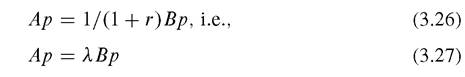
The alternative approach is a cyclic network of production. This idea is essential when we refer to a recyclic network. So far, we have considered the reproducibility of the production system. Here, the property of the input-output matrix bi — ai will play a decisive role in guaranteeing its reproducibility. Once the desired property of reproducibility—for example, the irreducible input matrix—has been established, the system will be replicated over time, by taking a certain price-cost system p = (p1, ■■■, pn/ supporting the productive circulation of input-output exchanges: 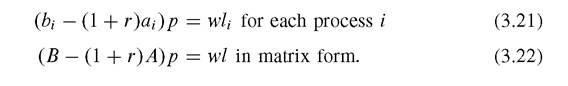
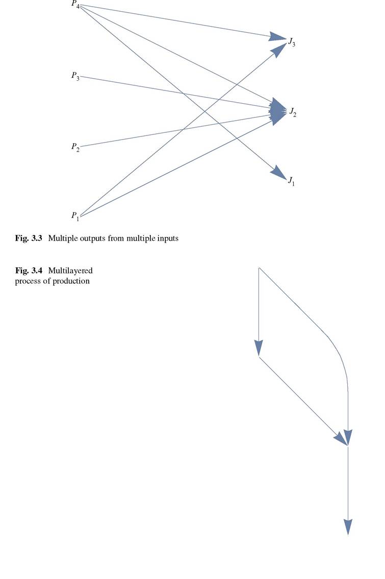
Table 3.2 Three-component table
| Primary | Secondary | Tertiary | Final demand | Export | Import | Domestic production | |
| Primary industry | 2 | 8 | 1 | 4 | 0 | -2 | 13 |
| Secondary industry | 3 | 175 | 58 | 156 | 56 | -59 | 388 |
| Tertiary industry | 2 | 75 | 143 | 344 | 17 | -11 | 570 |
| Good value added | 7 | 139 | 369 | ||||
| Domestic production | 13 | 388 | 570 |
Note 1: Unit: trillion yen
Note 2: The vertical direction represents the cost composition of the merchandise, and the horizontal direction the sales destination of the merchandise
Here r is the interest rate, wi the wage rate, and li the labor input.
Given an effective demand d =.d1, ■■■, dn/, this manipulation is justified by finding:
Conversely, it will not hold if the particular price system does not happen. The idea of the optimal price system has therefore rather shut off the dynamic properties of interactive activities. Once the equilibrium price system has been established, the system is potentially fixed by the equilibrium forever.
Finally, we show the empirically estimated network by the model form of the input-output table (basic input-output table) for Fiscal 2005 (Three-Component Table) (Table 3.2).[42]
The eigenvector centrality in the Three-Component Table, measured in 2005, is given as:

The inter-industrial relationship appearing in the input-output table often exhibits the all-entering properties of the matrix in a strict sense (Fig. 3.5).[43] The eigenvector centrality is inclined to be egalitarian. Instead of employing the eigenvector centrality, we can characterize the system by the closeness centrality of this three- character fundamental inter-industrial network:

This is shown as a highlighted graph in Fig. 3.6.
Fig. 3.5 The weighted adjacency graph of Table 3.2
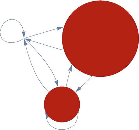
Fig. 3.6 The closeness centrality of Table 3.2
3.3.2 Criticism of the Traditional Approach
This formulation can be solved using the Duality Theorem of Linear Programming, but optimal solutions are often combined with a single industry operation. It is easily verified by simulation that the most profitable process is a simple one like oil production, not a more complex combination of multiple inputs.
This may be why oil-producing countries often have high GDP per capita. This is also seen in international trade theory. Optimization will tend to make the most profitable process a simple one with just a few inputs. A more complex process cannot necessarily become more profitable. As long as we adopt the method of optimization in choosing technique, therefore, we will be unable to discuss how a complex system of production could be organized and evolve, so it may be wise to abandon the assumption of an artificial optimal/equilibrium price system.We have, however, a useful insight from the traditional approach. Specifically, following Sraffa (1960), we can focus on the use of eigenvectors in the linear production system. In the 1930s, Sraffa was ready to identify the maximal (or principal) non-negative eigenvector with the invariant measure of the production of commodities by means of commodities. Sraffa happened to find virtually the same content as the Perron-Frobenius Theorem on the nonnegative eigenvectors on a real square matrix.[44] In his own economic modeling. Given a linear production system, we can find it uniquely, by fulfilling some conditions for a net producible system. We will then encounter the same property as the largest eigenvector, where the composition of industries on the input side is proportionate to that on the output side. If w is set as 0, we get:
This is the eigenvector equation if B is a unit matrix I. In the following, for simplicity, we assume B = I.
3.3.2.1 A Numerical Example
For convenience, we use a numerical example. We specify the numerical values in an input matrix A: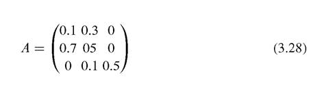
This input system can be net producible, i.e., produce a net surplus. This matrix has the eigenvectors and eigenvalues:
Eigenvectors:
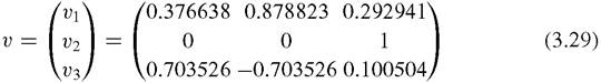
associated with eigenvalues:

The largest positive eigenvector is judged to be the first mode vι, as it has the largest eigenvalue u1 (scalar).
In this view of eigenvectors, the second sector in the first mode will give the dominant incidence of the system. According to Sraffa’s insight, this system’s valuation will not be affected by any disturbance of distributional factors, as long as the system is reduced to the eigen-system maintaining the proportionality between the input and output components. In other words, the largest eigenvector will behave like a fixed point as distributional variables r and w fluctuate. In our example, we measure the system by the composite commodity defined by the first mode vi, but not by a simple component like wheat. In this case, therefore, the second sector must be influential among the sectors used for valuation. However, this idea will also remove any opportunities for the production system to evolve.The input coefficients represent demand links; that is to say, aij means sector i requires j for self-activation. We may then regard our input matrix A as a weighted adjacency matrix, and it may represent the next productive (interindustrial) network.
Each vertex is regarded as a production sector or process of production. This network is easily verified using a cyclic graph.
We can therefore apply the cyclic network to the eigenvector centrality. By taking the transpose of matrix A, i.e., an adjacency matrix, the eigenvector centrality x may be calculated:
Here A0 is the transpose of matrix A. In economic terms, A0 represents supply links, while A represents demand links. x represents an eigenvector in terms of the activity level of the sector. We have already seen that the largest eigenvector of the input matrix is:

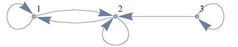
Fig. 3.8 Eigenvector centrality
Fig.
3.7 The cyclic network of the numerical example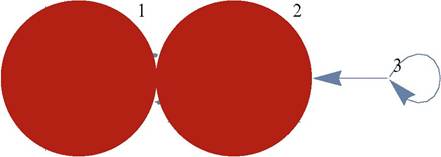
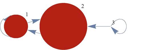
Fig. 3.9 Degree centrality
The largest eigenvector of the adjacency matrix turns out to be:
We have previously called the discrepancy between the input matrix and its transposed matrix the dual instability between the price system p and the quantity system x. Now we have again encountered the same kind of problems in terms of the network analysis. If we look only at valuation, the second sector incidence in our numerical example will be the largest. However, if we look at eigenvector centrality, the first and second sectors will be equally attractive. In other words, the network incidence in terms of the weighted adjacency matrix indicates that the first and second modes have equal incidences. The modes do not correspond exactly to the actual sectors, but each mode is constituted by the actual sector components (Figs. 3.7, 3.8, and 3.9).
We then discover that degree centrality is located on:
We therefore obtain a similar result for the demand links (the input matrix), in terms of ordering between the sectors.
We pointed out above that using the largest eigenvalue as the invariant measure might prevent any opportunities for the production system to evolve. However, the stability of the demand links differs from that of the supply links. This divergence will generate some dilemmas, because the given supply link will not necessarily support new demand links, if any should be created to a particular node. Node creating will affect the demand and supply links differently. We focus on the way the network will evolve by using some numerical examples.
3.4