The Historical Background to Network Thinking in Economic Theory
Looking back through the literature, several scholars have discussed linear production systems similar to the von Neumann model, including Leontief (1966), Sraffa (1960), and Walras (1874).
Sraffa’s contribution is perhaps especially important,because he analytically formulated the joint-productive recyclic system at almost the same time as von Neumann formulated his system. One criterion adopted by Sraffa was given by a set of macroeconomic distributive factors, including profit and wage rate.
It is easy for us to understand the inter-industrial input-output table as a network analysis. In the mid-twentieth century, many scholars worked on linear production systems, in view of the inequality approach. This is typically represented as the Duality Theorems of Systems of Linear Inequalities. These were believed to advocate an idea of equilibrium price in the context of the inter-industrial production system. However, we are now confronted by a constant process of innovation in the real world. Nevertheless, the idea of optimal prices guaranteed by the Duality Theorems merely freezes all the renovating processes of production, because the system can be fixed forever once the equilibrium price system has been attained. In other words, the idea of the optimal price system has rather shut off the dynamic properties of interactive activities. We should therefore examine again the approach to inter-industrial productive systems as part of a network analysis.
Georg Friedrich List (1789-1846) developed the idea of a national system of innovation. Arthur (2009) recommended national competitiveness in view of path dependency. By taking two instances, i.e., the power transmission line and hydroelectric power plants, Klaus Mainzer recently pointed out two industrialists who had successfully developed network thinking[40]:
Oskar von Miller (1855-1934), a German engineer who founded the Deutsches Museum.
Walter Rathenau (1867-1922), the founder of Allgemeine Elektrizitats- Gesellschaft (AEG), an electrical-engineering company, and foreign minister responsible for the Rapallo Treaty.
From this point of view, productive networks must be hierarchical, and their analysis will need complexity theory. This is explained further in Chap. 5. Here, we consider only the recycling of production.
3.2.1 TheRecyclingofProduction
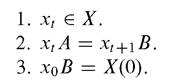
Figure 3.1 depicts a recycling system of production. In a real system of human production, each link of the recycling chain, i.e., each production process, must be currently associated with each labor input. If we remove an edge-node within the recycling operation in the figure, the system may degenerate into another one. This operation is called “truncation” and is the same as the procedure of rewiring nodes. However, we will need a more sophisticated rule than the assortative/dissortative one argued above. In Fig. 3.1, an addition of a new mode in the left diagram can give rise amore complicated relationship.
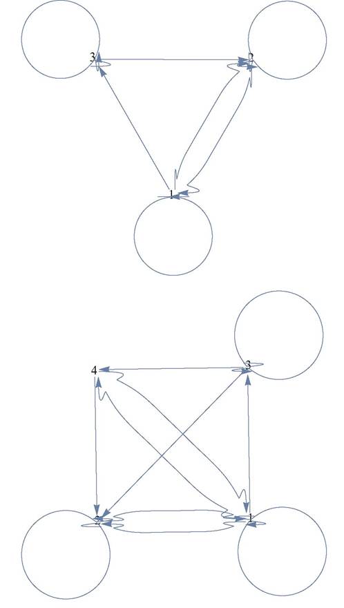
Fig. 3.1 Productive networks
3.2.2 The von Neumann Economy
We define the admissible set of activities X in the von Neumann model of production as:
An activity mix is the mixed strategy that satisfies the above admissible set X. We denote the time series of feasible programs by Xe, and the time series of chosen programs by Ce:
The feasible programs are technologically bounded by the upper limit, so the maximal welfare level will be guaranteed.
3.2.3 Von Neumann’s Original Formulation
The economic system of production consists of dual systems of price and quantity. Production is achieved through a recycling network. In classic economics, we call this type of production “inter-industrial reproduction”.
As a brief illustration, the production of outputs by recycling is taken to be achieved by a set of production processes by employing human labor and materials obtained from the outputs themselves. A productive process i is therefore described as:
ai is a set of materials aij for process (or activity) i, li is a labor input essential for process i, and bi is a set of outputs bij contributed by process (or activity) i.
 is an input matrix,
 is an output matrix and
 is a labor
vector. We can impose regularity conditions on our production system to guarantee solutions. We must then have a price system as the valuation measure of price, and a quantity system as the technically feasible activity measure:
Here pj represents the price of commodity j and qi is an activity level i, which together construct evaluation systems that are the price-cost and supply-demand equation systems.
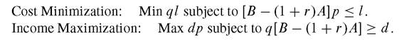
3.2.4 Classical Truncation Rules of Choice of Techniques
We define two types of feasibility: price and quantity.[41] Price feasibility is defined as:
Price feasibility: Whether the price-cost equation of a subsystem is fulfilled with respect to non-negative prices at a given rate of profit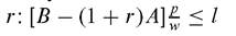
This means that sales minus input costs (including interest payments) is less than labor cost wl.
Quantity feasibility is defined as:
Quantity feasibility: Whether the demand-supply equation of a subsystem is fulfilled with respect to non-negative activities at a given rate of growth g:
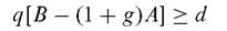
Here dj represents a final demand of j consumed by labor.
We call d = (di) a final demand or consumption vector. This means that supply minus intermediate input (with growth factor added) is greater than final demand.Now truncation rules depend on:
3.2.5 Adaptive Plans in the von Neumann Economy
The society that chose c^ can uniquely specify the welfare level u(c/. For convenience, this may be regarded as the expected net output or profit. In this case, we use the von Neumann payoff function as the welfare level. The welfare level that the program θ accumulates during the period (0, T) is then:
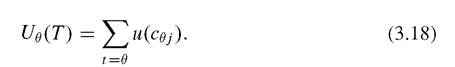
Program θ is preferred to any other program θ' if:
The optimal program is θ, satisfying the condition: 
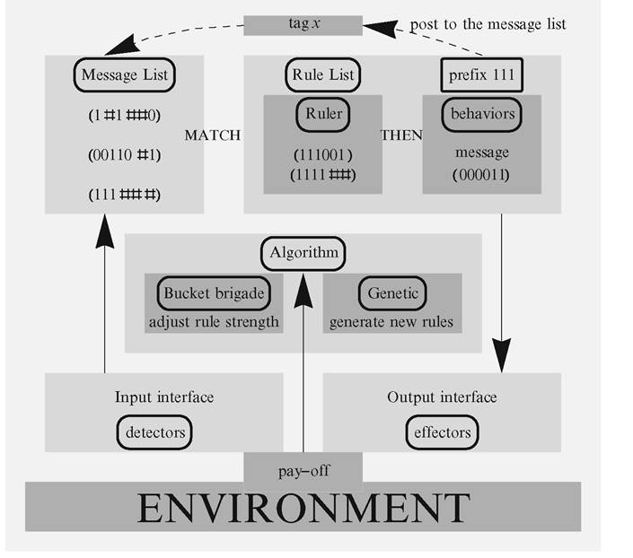
Fig. 3.2 The classifier system
An adaptive plan τ is such that a production program C⅛ is chosen on the basis of information received from the economy (E, the environment). The problem is choosing a particular adaptive plan approaching an optimal program in a broader domain of the environment (Fig. 3.2).
3.2.6 The Market Mechanism as a Genetic Algorithm
We noticed earlier that the bid/ask mechanism for selecting an adaptive productive plan or program might be replaced by the bucket brigade algorithm as an internal mechanism. The process based on the evolutionary genetic algorithm moves to a new stage via a feedback loop from a consecutively modified environment. The environment in the genetic algorithm is interpreted as an environmental niche, according to Holland (1992, p. 11; 1995, pp. 22-27).
Thefield might be strategically chosen for the agents. This is called stage-setting in a genetic algorithm. Under such an implementation of the environmental niche, the environment for agents in this sense does not settle at a given landscape. Hence, the economic system will not necessarily be bound to an equilibrium state in which equilibrium prices dominate (Aruka 2012).3.2.2 A System’s Eigenvector to Measure the Profitability of the Fictitious Processes/Commodities
Suppose the actual production system to be a general joint-production system. The system does not necessarily confirm its general solution.
3.2.3 Minimum Spanning Trees of the Industrial Network
In mathematical terms, a spanning tree of a connected and undirected graph is one that includes and connects all the graph’s vertices. The Minimum Spanning Tree (MST) is the smallest possible spanning tree for that graph. We can derive the MST from the cross-correlation matrices. Its diameter is the largest number of links that must be traversed to get from one node to another. This measurement gives an important index to monitor the transition between the different phases. The industry cluster may be regarded as more open if the degree of an MST is larger. By this definition, it follows that financial contagion spreads faster on a closer MST, and positive sentiment on a more open one.
3.2.8.1 Hub Industries in Japan
Cheong et al. (2012) discovered from the MST formations for each time period that the Chemicals and Electric Machinery industries are consistently the hubs through all five macroeconomic periods (Table 3.1). The authors also reached an interesting conclusion that “Going through all eight MSTs, we see that the growth hubs are fairly robust and persistent, and recover rapidly after short disappearances. The quality hubs, on the other hand, do not survive for very long. We take this to mean that Japanese investors are actually more optimistic than most people give them credit for”.
Table 3.1 Cross-correlations between the 36 Nikkei 500 Japanese industry indices over a 14-year period encompassing five macroeconomic periods
| Minimum | Average | Maximum | MST diameter | |
| Entire time series | 0.216 | 0.507 | 0.805 | 5 |
| Asian financial crisis (1997-1999) | 0.234 | 0.485 | 0.767 | 5 |
| Technology bubble crisis (2000-2002) | 0.115 | 0.509 | 0.836 | 10 |
| Economic growth (2003-2006) | 0.126 | 0.498 | 0.819 | 9 |
| Subprime crisis (2007-2008) | 0:284 | 0.66 | 0.918 | 8 |
| Lehman brothers crisis (2008-2010) | 0.259 | 0.63 | 0.919 | 8 |
Source: Cheong et al.
(2012). http://dx.doi.org/10.5018/economics-ejournal.ja.2012-5
3.3