Endogenous fluctuations
In the models reviewed so far, the economies converge in the long run to balanced- growth equilibria characterized by linear dynamics. Growth models with expanding variety and technological complementarities can, however, generate richer long-run dynamics, including limit cycles.
In this section, we review two such models.In the former, based on Matsuyama (1999), cycles in innovation and growth arise from the deterministic dynamics of two-sector models with an endogenous market structure. The theory can explain some empirical observations about low-frequency cycles, and their interplay with the growth process. In particular, it predicts that waves of rapid growth mainly driven by “factor accumulation” are followed by spells of innovation- driven growth. Interestingly, these latter periods are characterized by lower investments and slower growth. This is consistent with the findings of Young (1995) that the growth performance of East-Asian countries was mainly due to physical and human capital accumulation, while there was little total factor productivity (TFP) growth. According to Matsuyama’s theory, the observation of low TFP growth should not lead to the pessimistic conclusions that growth is destined to die-off. Rather, rapid factor accumulation could set the stage for a new phase of growth characterized by more innovative activity. The predictions of this theory bear similarities to those of models with General Purpose Technologies (GPT), e.g., Helpman (1998) and Aghion and Howitt (1998, Chapter 8). For instance, they predict that a period of rapid transformation and intense innovation (e.g., the 1970’s) can be associated with productivity slowdowns. However, GPT-based theories rely on the exogenous arrival of new “fundamental” innovations generating downstream complementarities. In contrast, cycles in Matsuyama (1999) are entirely endogenous.[70]
In the latter model, based on Evans et al.
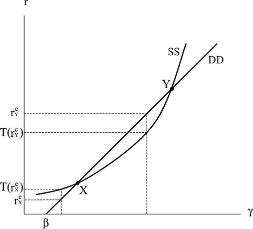
(1998), cycles in innovation and growth are instead driven by expectational indeterminacy. The mechanism in this paper is different, as cycles hinge on multiple equilibria and sunspots. Some main predictions are also different: contrary to Matsuyama (1999), the equilibrium features a positive comovement of investments and innovation. The main contribution of the paper is to show that cycles can be learned by unsophisticated agents holding adaptive expectations. Thus, the predictive power of the theory does not rest on the assumption that agents’ expectations are rational and that agents can compute complicated dynamic equilibria.7.1. Deterministiccycles
Matsuyama (1999) presents a model of expanding variety where an economy can perpetually oscillate in equilibrium between periods of innovation and periods of no innovation. Cycles arise from the deterministic periodic oscillations of two state variables (physical capital and knowledge). Unlike the model that will be discussed in the next section, the equilibrium is determinate and there are no multiple steady-states.
More specifically, the source of the oscillatory dynamics is the market structure of the intermediate goods market. Monopoly power is assumed to be eroded after one period. The loss of monopoly power is due to the activity of a competitive fringe which can copy the technology with a one-period lag. In every period, new industries are monopolized, while mature industries are competitive. The profits of innovators depend on the market structure of the intermediate sector. The larger is the share of competitive industries in the intermediate sector, the lower is the profit of innovative firms, since competitive industries sell larger quantities and charge lower prices. In periods of high innovation, a large share of industries are monopolized, which increases the profitability of innovation, thereby generating a feedback. In these times, investment in physical capital is low due to the crowding out from the research activity.
Conversely, times of low innovation are times of high competition, since old monopolies lose power and there are few new firms. Thus, the rents accruing to innovative firms are small. In these periods, savings are invested in physical capital, and while innovation is low, the high accumulation of physical capital creates the conditions for future innovation to be profitable.Time is discrete. The production of final goods is as in (3), where we set Ly = L = 1. Intermediate goods are produced using physical capital, with one unit of capital producing one unit of intermediate product, x. Innovation also requires capital, with a requirement of μ units of capital per innovation. Monopoly power is assumed to last one period only. Therefore, in period t, all intermediate inputs with an index z ∈ [0, At-1]
can decide to time the implementation of innovations [similarly to Shleifer (1986)]. In this model, agents time the implementation so as to profit from buoyant demand and maximize the duration of their leadership. This mechanism leads to a clustering of innovations and endogenous cycles. While this model can explain some features of fluctuations at business cycle frequencies, Matsuyama’s model is better suited for the analysis of long waves.
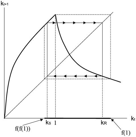
Figure 6.
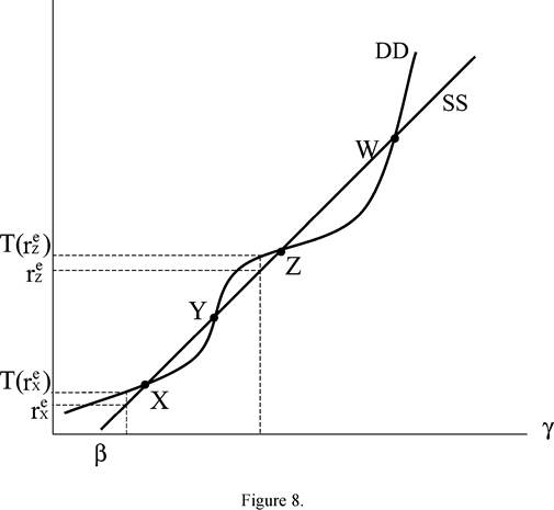
cycle is not necessarily stable, and if it is unstable, the economy can converge to cycles of higher periodicity or feature chaos. A general property of the dynamics is that the economy necessarily enters the region Iabs = [f (f (1)), f (1)] (shaded in Figure 6), and never escapes from it.[71]
In the case described by Figure 6, the model predicts that a poor economy would first grow through capital accumulation, and eventually enter the absorbing region Iabs.
Then, there is an alternation of periods of innovation and periods of no innovation. GDP per capita grows on average, but at a non-steady rate, and there are cycles in the innovative activity. Interestingly, output and capital grow more quickly in periods of no innovation (Solow regime) than in periods of high innovation (Romer regime). Another implication is that if an economy grows quickly, but has a low TFP growth, this does not imply that growth will die-off. Rather, fast capital accumulation can create the conditions for future waves of innovation, and vice versa.7.2. Learningandsunspots
Evans et al. (1998) propose the following generalization of the technology (3) for final production:

where ζφ = α. This specification encompasses the technology (3), in the case of φ = 1, and allows intermediate inputs to be complements or substitutes. They focus on the case of complementarity (φ > 1), and show that in this case, the equilibrium can feature multiple steady states, expectational indeterminacy and sunspots. They emphasize the possibility of equilibria where the economy can switch stochastically between periods of high and low growth.
Time is discrete, and intermediate firms rent physical capital from consumers to produce intermediate goods. One unit of capital is required per unit of intermediate good produced. Capital is assumed not to depreciate. The resource constraint of this economy is:
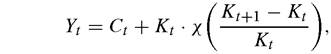
where χ(.) is a function such that χ' > 0, χ" φ 0. If there are no costs of adjustment, then, χ(x) = x.If χ " > 0, there are convex costs of adjustments.
By proceeding as in Section 2, we can characterize the equilibrium of the intermediate industry.59 The profit of intermediate producers, in particular, turns out to be:
[1] Note that firms rent, and do not own, their capital stock.
Adjustment costs are borne at the aggregate level, not at the level of each decision unit. Therefore, it continues to be legitimate to write the profit maximization problem for intermediate producers as a sequence of static maximization problems.
The model assumes increasing returns to physical and knowledge capital. The reduced form representation of the final good technology is:
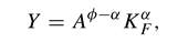
where Kf = Ax denotes aggregate capital used in intermediate production. Empirical estimates suggest that α ≤ 0.4, which implies that the lower bound to the output elasticity of knowledge to generate multiplicity is φ — α = 0.6. Evans et al. (1998) provide a numerical example of an E-stable sunspot equilibrium, assuming φ = 4. Recent estimations from Porter and Stern (2000) using patent numbers report φ — α to be around 0.1, however. Therefore, the model seems to require somehow extreme parameters to generate endogenous fluctuations.
Augmenting the model with other accumulated assets, such as human capital, may help obtain the results under realistic parameter configurations. This is complicated by the presence of scale effects in the expanding variety model. However, in a recent paper, Dalgaard and Kreiner (2001) formulate a version of the model with human capital accumulation and without scale effects. In their model, both human capital (embodied knowledge) and technical change (disembodied knowledge) are used to produce final goods. The scale effect is avoided by congestion effects in the accumulation of human capital. An interesting feature of this model is that, unlike other recent models without scale effects, positive long-run growth in income per capita does not hinge on positive population growth.
8.